本章对Transformer在计算机视觉中的算法和应用做了原理介绍和效果展示。

10. Vision Transformers

10.1 初版Vit

1、整体概览

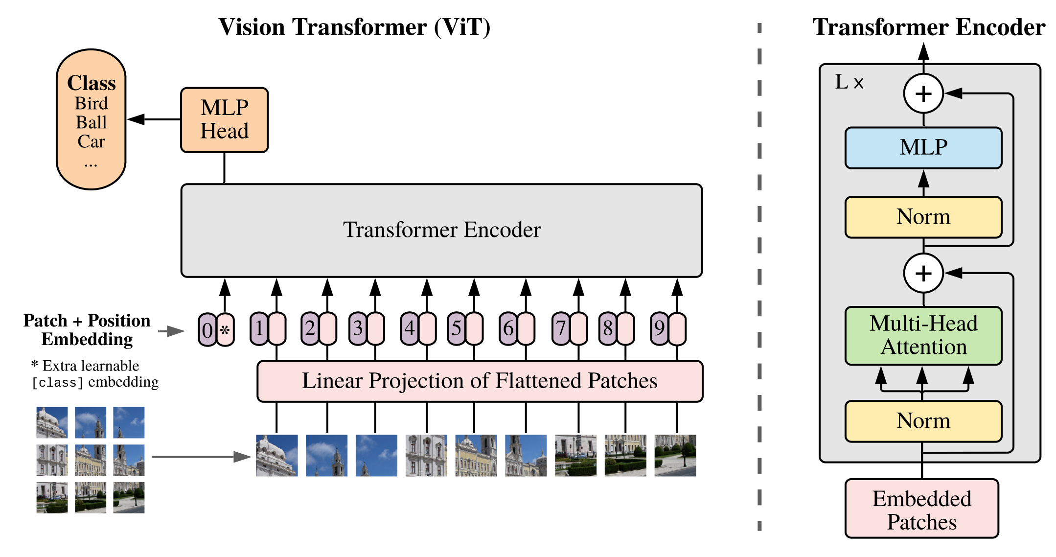
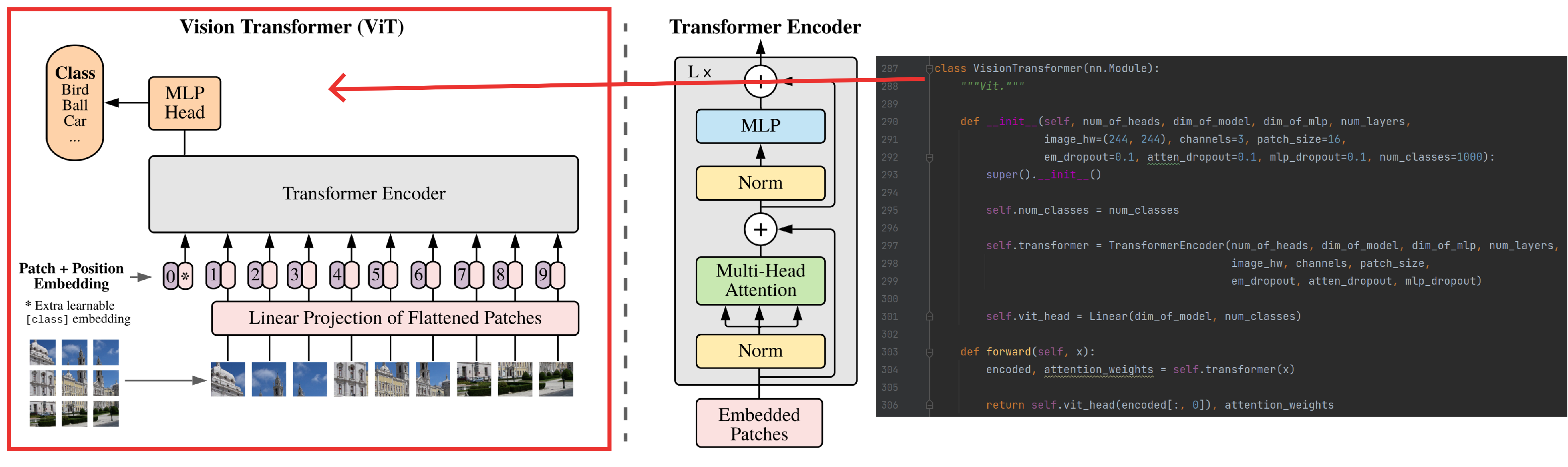
第一次将Transformer机制引入CV领域（准确的说是图像分类）的是Google Brain的Neil Houlsby, Alexey Dosovitskiy等人在ICLR 2021提交的《An Image is Worth 16*16 Words: Transformers for Image Recognition at Scale》一文，本节对这篇文章做个概要介绍。

ViT用于图像分类有以下优缺点，优点：完全不使用CNN结构，自然也就避免了CNN的缺点、在分类效果上甚至好于CNN类模型（如：ResNet）；缺点：需要比较大的数据集生成预训练模型、在新任务上做fine-tuning时要特别小心、想效果好，模型要很大。

ViT整体结构我认为比较原汁原味的继承了NLP中的Transformer，所以原理没什么好重复讲的，更多的是在做实验。

通用的结构包括：

具有标准Multi-Head Self-Attention的Transformer encoder
Channel方向做归一化的Layer norm
位置编码Position embeddings。

个性化的结构包括：

由于标准Transformer接收1维序列，所以需要把2维的图片通过等大小切片并横向拼接转化为1维序列，即：假设原始图片大小为：$H×W×C$，每个切片分辨率大小为$P×P$，则一共会有$N=HW/P^2$个切片，输入序列patch embeddings维度为：$N×(P^2\cdot C)$。
类似BERT，通过embedding一个class token（下图中加*的部分），来“概括”整幅图的语义表示，从而用于下游分类任务。
Transformer encoder后面接一个多层感知机层(MLP layer)。

ViT运转过程如图：

动图来源于这里网络结构如图：

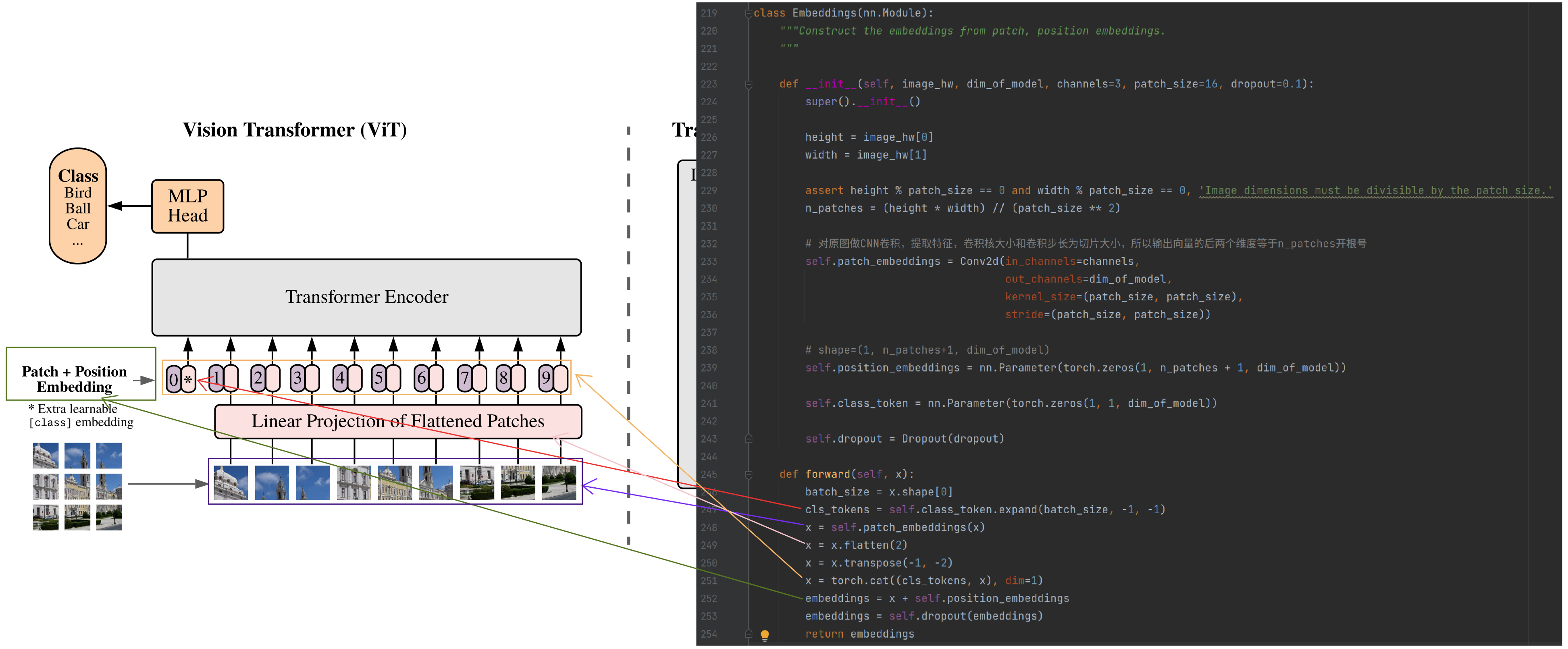
2、代码实践

Embedding
整个过程分几步：切片、引入class token、切片铺平、与位置编码相加，过程如下：
1、需要确保图片长×宽可以整除切片大小，例如，图片为224×224、切片大小为16×16，则满足要求
2、通过对原图做CNN卷积得到切片（patch），并把切片铺平
3、把class token向量拼接到切片铺平后的向量的最前面位置
5、将第3步得到的向量与位置编码向量相加，用dropout做下正则化后返回
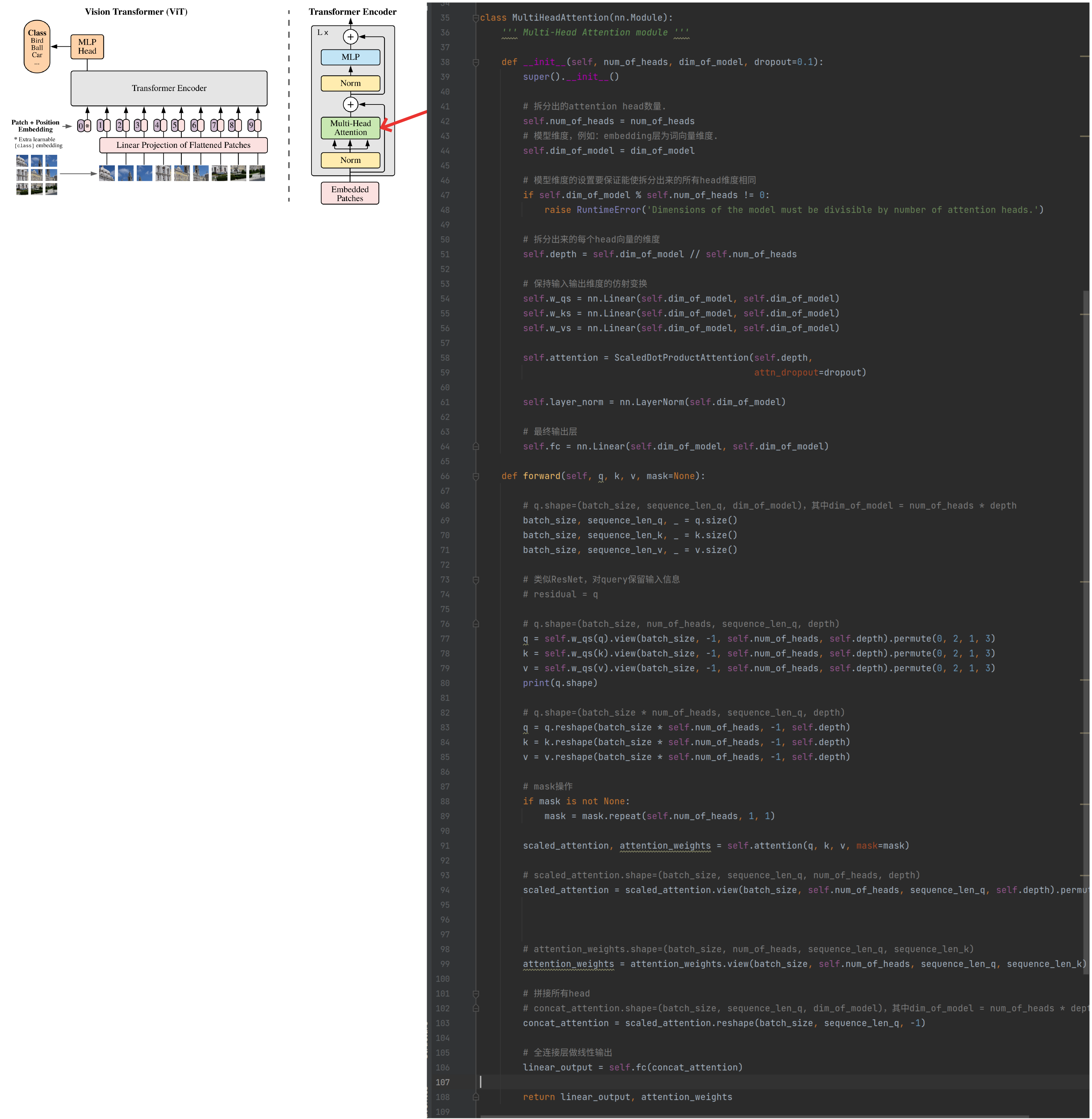
MultiHeadAttention
稍作修改，把Normlayer去掉，沿用之前在第六章介绍的MultiHeadAttention结构，如下图：
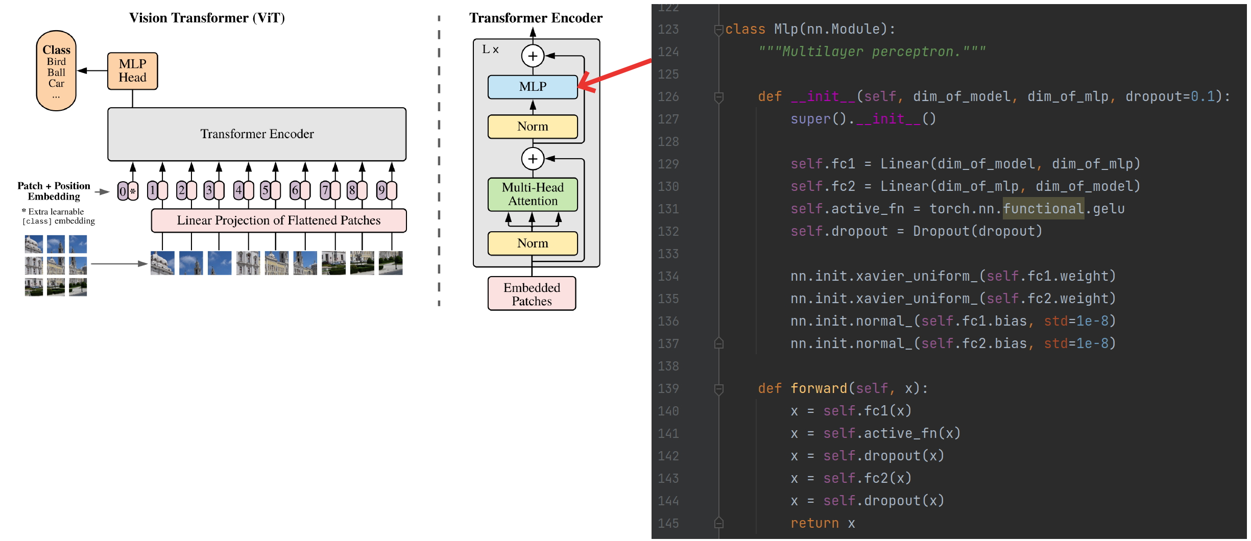
MLP
使用BERT中的GELU激活函数，并构建一个两层感知机，如下图：
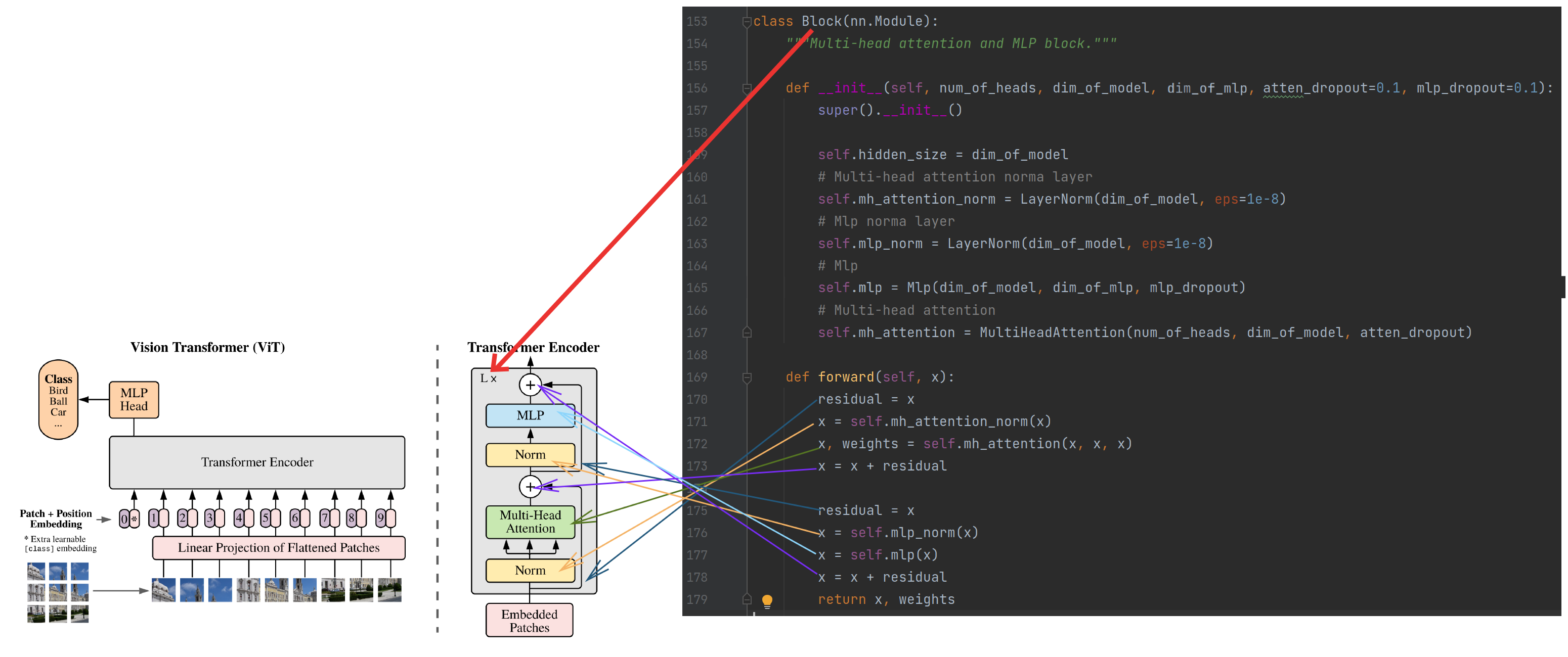
Block
组合Normlayer、MultiHeadAttention和MLP，得到一个基础的、可复制多个的最小Block结构，如下图：
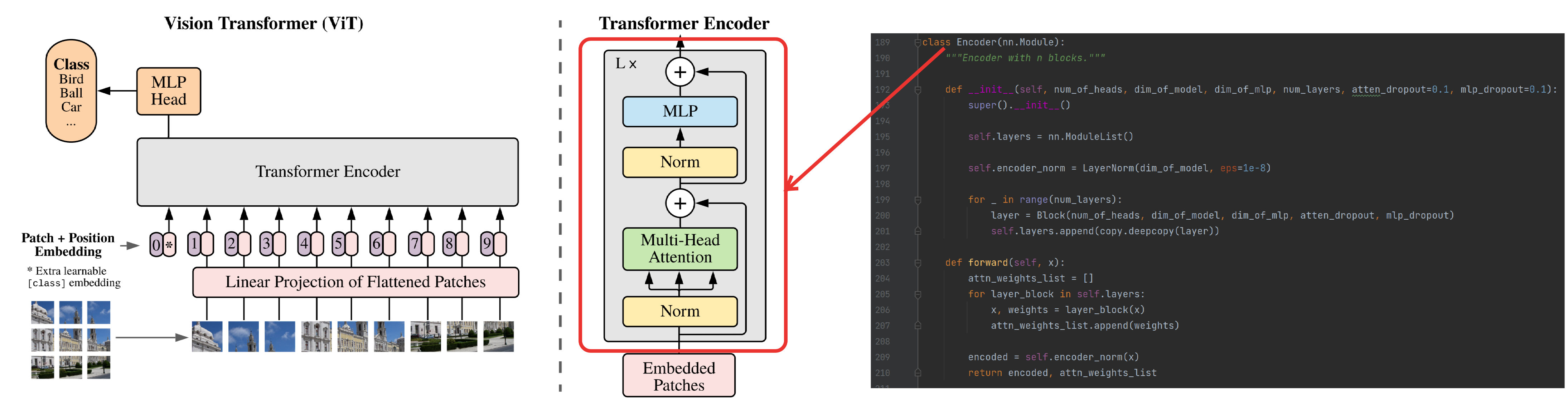
Encoder
若干个Block组成一个Encoder，如下图：
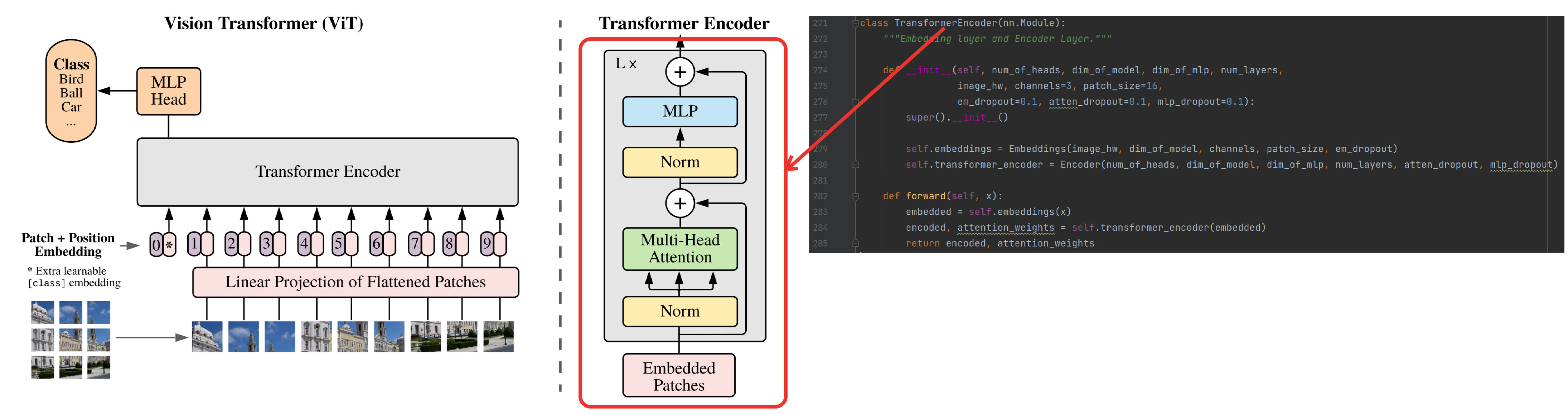
TransformerEncoder
Embedding和Encoder共同组合成Transformer Encoder结构，如下图：

VisionTransformer

构建一个用于多分类的vision transformer，如下图：

以上过程的完整代码如下：

import numpy as np
import torch
import torch.nn as nn
from torch.nn import Dropout, Linear, Conv2d, LayerNorm
import copy


class ScaledDotProductAttention(nn.Module):
    ''' Scaled Dot-Product Attention '''

    def __init__(self, d_k, attn_dropout=0.1):
        super().__init__()
        # 缩放因子
        self.scalar = 1 / np.power(d_k, 0.5)
        self.dropout = nn.Dropout(attn_dropout)
        self.softmax = nn.Softmax(dim=2)

    def forward(self, q, k, v, mask=None):
        # 计算q∙k
        attn = torch.bmm(q, k.transpose(1, 2))
        # 计算q∙k/sqr(d_k)
        attn = attn * self.scalar

        # attention masked
        if mask is not None:
            attn = attn.masked_fill(mask.bool(), -np.inf)

        # 计算softmax(q∙k/sqr(d_k))
        attn = self.softmax(attn)
        attn = self.dropout(attn)
        # 计算softmax(q∙k/sqr(d_k))∙v
        sdp_output = torch.bmm(attn, v)

        return sdp_output, attn


class MultiHeadAttention(nn.Module):
    """ Multi-Head Attention module """

    def __init__(self, num_of_heads, dim_of_model, dropout=0.1):
        super().__init__()

        # 拆分出的attention head数量.
        self.num_of_heads = num_of_heads
        # 模型维度，例如：embedding层为词向量维度.
        self.dim_of_model = dim_of_model

        # 模型维度的设置要保证能使拆分出来的所有head维度相同
        if self.dim_of_model % self.num_of_heads != 0:
            raise RuntimeError('Dimensions of the model must be divisible by number of attention heads.')

        # 拆分出来的每个head向量的维度
        self.depth = self.dim_of_model // self.num_of_heads

        # 保持输入输出维度的仿射变换
        self.w_qs = nn.Linear(self.dim_of_model, self.dim_of_model)
        self.w_ks = nn.Linear(self.dim_of_model, self.dim_of_model)
        self.w_vs = nn.Linear(self.dim_of_model, self.dim_of_model)

        self.attention = ScaledDotProductAttention(self.depth,
                                                   attn_dropout=dropout)

        self.layer_norm = nn.LayerNorm(self.dim_of_model)

        # 最终输出层
        self.fc = nn.Linear(self.dim_of_model, self.dim_of_model)

    def forward(self, q, k, v, mask=None):

        # q.shape=(batch_size, sequence_len_q, dim_of_model)，其中dim_of_model = num_of_heads * depth
        batch_size, sequence_len_q, _ = q.size()
        batch_size, sequence_len_k, _ = k.size()
        batch_size, sequence_len_v, _ = v.size()

        # 类似ResNet，对query保留输入信息
        # residual = q

        # q.shape=(batch_size, num_of_heads, sequence_len_q, depth)
        q = self.w_qs(q).view(batch_size, -1, self.num_of_heads, self.depth).permute(0, 2, 1, 3)
        k = self.w_qs(k).view(batch_size, -1, self.num_of_heads, self.depth).permute(0, 2, 1, 3)
        v = self.w_qs(v).view(batch_size, -1, self.num_of_heads, self.depth).permute(0, 2, 1, 3)
        print(q.shape)

        # q.shape=(batch_size * num_of_heads, sequence_len_q, depth)
        q = q.reshape(batch_size * self.num_of_heads, -1, self.depth)
        k = k.reshape(batch_size * self.num_of_heads, -1, self.depth)
        v = v.reshape(batch_size * self.num_of_heads, -1, self.depth)

        # mask操作
        if mask is not None:
            mask = mask.repeat(self.num_of_heads, 1, 1)

        scaled_attention, attention_weights = self.attention(q, k, v, mask=mask)

        # scaled_attention.shape=(batch_size, sequence_len_q, num_of_heads, depth)
        scaled_attention = scaled_attention.view(batch_size, self.num_of_heads, sequence_len_q, self.depth).permute(0,
                                                                                                                    2,
                                                                                                                    1,
                                                                                                                    3)
        # attention_weights.shape=(batch_size, num_of_heads, sequence_len_q, sequence_len_k)
        attention_weights = attention_weights.view(batch_size, self.num_of_heads, sequence_len_q, sequence_len_k)

        # 拼接所有head
        # concat_attention.shape=(batch_size, sequence_len_q, dim_of_model)，其中dim_of_model = num_of_heads * depth
        concat_attention = scaled_attention.reshape(batch_size, sequence_len_q, -1)

        # 全连接层做线性输出
        linear_output = self.fc(concat_attention)

        return linear_output, attention_weights


# (num_of_heads, dim_of_model)
mha = MultiHeadAttention(12, 768)

# (batch_size, sequence_len_q, dim_of_model)
q = torch.Tensor(32, 197, 768)

output, attention_weights = mha(q, k=q, v=q, mask=None)

print('shape of output:"{0}", shape of attention weight:"{1}"'.format(output.shape, attention_weights.shape))


class Mlp(nn.Module):
    """Multilayer perceptron."""

    def __init__(self, dim_of_model, dim_of_mlp, dropout=0.1):
        super().__init__()

        self.fc1 = Linear(dim_of_model, dim_of_mlp)
        self.fc2 = Linear(dim_of_mlp, dim_of_model)
        self.active_fn = torch.nn.functional.gelu
        self.dropout = Dropout(dropout)

        nn.init.xavier_uniform_(self.fc1.weight)
        nn.init.xavier_uniform_(self.fc2.weight)
        nn.init.normal_(self.fc1.bias, std=1e-8)
        nn.init.normal_(self.fc2.bias, std=1e-8)

    def forward(self, x):
        x = self.fc1(x)
        x = self.active_fn(x)
        x = self.dropout(x)
        x = self.fc2(x)
        x = self.dropout(x)
        return x


mp = Mlp(768, 3072)
r = mp(output)
print('shape of mlp:"{0}""'.format(r.shape))


class Block(nn.Module):
    """Multi-head attention and MLP block."""

    def __init__(self, num_of_heads, dim_of_model, dim_of_mlp, atten_dropout=0.1, mlp_dropout=0.1):
        super().__init__()

        self.hidden_size = dim_of_model
        # Multi-head attention norma layer
        self.mh_attention_norm = LayerNorm(dim_of_model, eps=1e-8)
        # Mlp norma layer
        self.mlp_norm = LayerNorm(dim_of_model, eps=1e-8)
        # Mlp
        self.mlp = Mlp(dim_of_model, dim_of_mlp, mlp_dropout)
        # Multi-head attention
        self.mh_attention = MultiHeadAttention(num_of_heads, dim_of_model, atten_dropout)

    def forward(self, x):
        residual = x
        x = self.mh_attention_norm(x)
        x, weights = self.mh_attention(x, x, x)
        x = x + residual

        residual = x
        x = self.mlp_norm(x)
        x = self.mlp(x)
        x = x + residual
        return x, weights


b = Block(12, 768, 3072)
q = torch.Tensor(32, 197, 768)
output, attention_weights = b(q)
print('shape of output:"{0}", shape of attention weight:"{1}"'.format(output.shape, attention_weights.shape))


class Encoder(nn.Module):
    """Encoder with n blocks."""

    def __init__(self, num_of_heads, dim_of_model, dim_of_mlp, num_layers, atten_dropout=0.1, mlp_dropout=0.1):
        super().__init__()

        self.layers = nn.ModuleList()

        self.encoder_norm = LayerNorm(dim_of_model, eps=1e-8)

        for _ in range(num_layers):
            layer = Block(num_of_heads, dim_of_model, dim_of_mlp, atten_dropout, mlp_dropout)
            self.layers.append(copy.deepcopy(layer))

    def forward(self, x):
        attn_weights_list = []
        for layer_block in self.layers:
            x, weights = layer_block(x)
            attn_weights_list.append(weights)

        encoded = self.encoder_norm(x)
        return encoded, attn_weights_list


encoder = Encoder(12, 768, 3072, 1)
q = torch.Tensor(32, 197, 768)
output, attention_weights = encoder(q)
print('shape of output:"{0}", shape of attention weight:"{1}"'.format(output.shape, attention_weights[0].shape))


class Embeddings(nn.Module):
    """Construct the embeddings from patch, position embeddings.
    """

    def __init__(self, image_hw, dim_of_model, channels=3, patch_size=16, dropout=0.1):
        super().__init__()

        height = image_hw[0]
        width = image_hw[1]

        assert height % patch_size == 0 and width % patch_size == 0, 'Image dimensions must be divisible by the patch size.'
        n_patches = (height * width) // (patch_size ** 2)

        # 对原图做CNN卷积，提取特征，卷积核大小和卷积步长为切片大小，所以输出向量的后两个维度等于n_patches开根号
        self.patch_embeddings = Conv2d(in_channels=channels,
                                       out_channels=dim_of_model,
                                       kernel_size=(patch_size, patch_size),
                                       stride=(patch_size, patch_size))

        # shape=(1, n_patches+1, dim_of_model)
        self.position_embeddings = nn.Parameter(torch.zeros(1, n_patches + 1, dim_of_model))

        self.class_token = nn.Parameter(torch.zeros(1, 1, dim_of_model))

        self.dropout = Dropout(dropout)

    def forward(self, x):
        batch_size = x.shape[0]
        cls_tokens = self.class_token.expand(batch_size, -1, -1)
        x = self.patch_embeddings(x)
        x = x.flatten(2)
        x = x.transpose(-1, -2)
        x = torch.cat((cls_tokens, x), dim=1)
        embeddings = x + self.position_embeddings
        embeddings = self.dropout(embeddings)
        return embeddings


emb = Embeddings((224, 224), 768)
q = torch.Tensor(32, 3, 224, 224)
r = emb(q)
print('shape of embedding:"{0}""'.format(r.shape))


class TransformerEncoder(nn.Module):
    """Embedding layer and Encoder Layer."""

    def __init__(self, num_of_heads, dim_of_model, dim_of_mlp, num_layers,
                 image_hw, channels=3, patch_size=16,
                 em_dropout=0.1, atten_dropout=0.1, mlp_dropout=0.1):
        super().__init__()

        self.embeddings = Embeddings(image_hw, dim_of_model, channels, patch_size, em_dropout)
        self.transformer_encoder = Encoder(num_of_heads, dim_of_model, dim_of_mlp, num_layers, atten_dropout,
                                           mlp_dropout)

    def forward(self, x):
        embedded = self.embeddings(x)
        encoded, attention_weights = self.transformer_encoder(embedded)
        return encoded, attention_weights


trans = TransformerEncoder(12, 768, 3072, 2, (224, 224))
q = torch.Tensor(32, 3, 224, 224)
r, _ = trans(q)
print('shape of transformer encoder:"{0}""'.format(r.shape))


class VisionTransformer(nn.Module):
    """Vit."""

    def __init__(self, num_of_heads, dim_of_model, dim_of_mlp, num_layers,
                 image_hw=(224, 224), channels=3, patch_size=16,
                 em_dropout=0.1, atten_dropout=0.1, mlp_dropout=0.1, num_classes=1000):
        super().__init__()

        self.num_classes = num_classes

        self.transformer = TransformerEncoder(num_of_heads, dim_of_model, dim_of_mlp, num_layers,
                                              image_hw, channels, patch_size,
                                              em_dropout, atten_dropout, mlp_dropout)

        self.vit_head = Linear(dim_of_model, num_classes)

    def forward(self, x):
        encoded, attention_weights = self.transformer(x)

        return self.vit_head(encoded[:, 0]), attention_weights


vit = VisionTransformer(12, 768, 3072, 2, (224, 224))
q = torch.Tensor(32, 3, 224, 224)
r, _ = vit(q)
print('shape of vision transformer:"{0}""'.format(r.shape))

from torchviz import make_dot
architecture = make_dot(r, params=dict(list(vit.named_parameters())))
architecture.format = "png"
architecture.directory = "data"
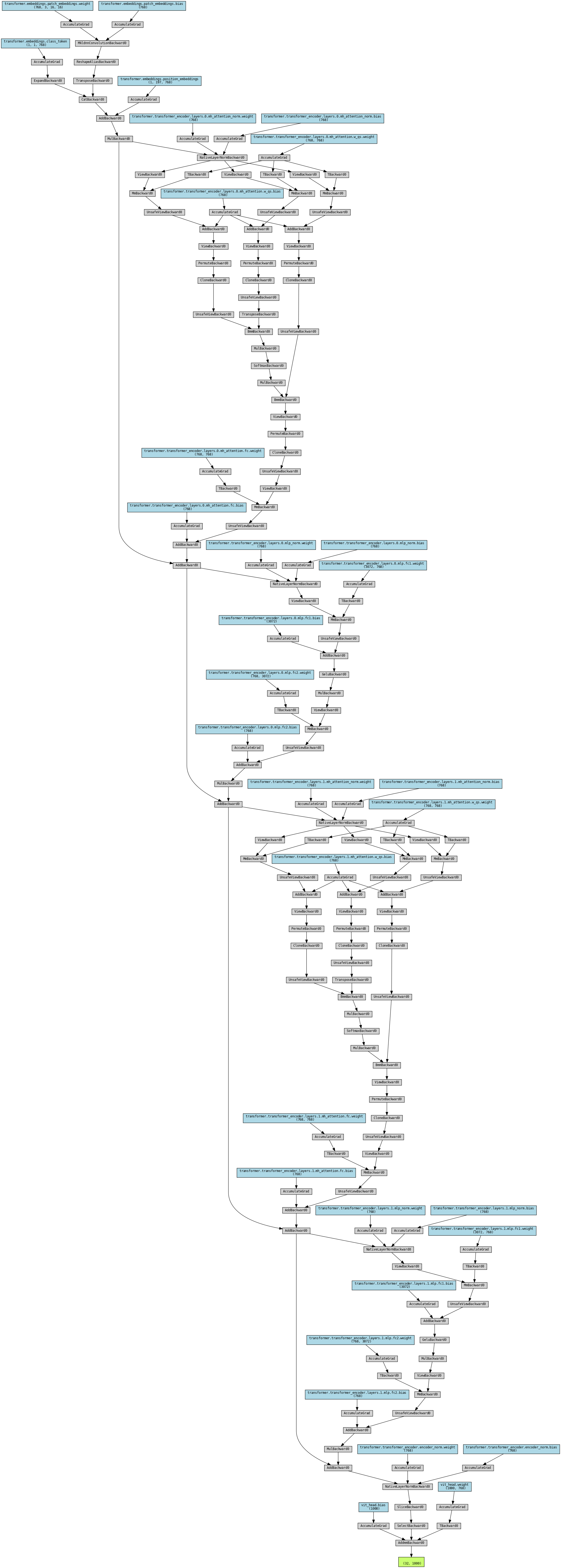
architecture.view()

假设，采用12个head，模型隐层维度为768，感知机维度为3072，block个数为2，图片大小为224×224，batch大小为32，则网络结构可视化后如下：

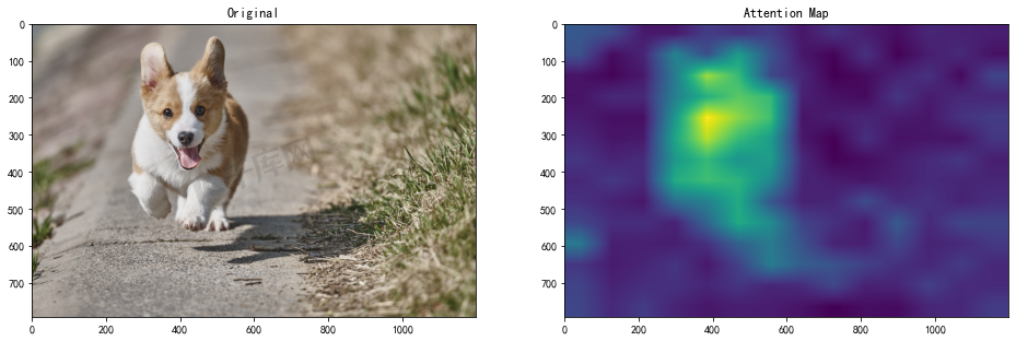
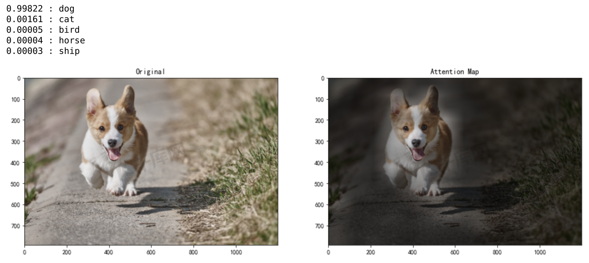
直观看个transformer机制在图像中的作用更有感觉：随着attention机制作用的层数越深，对柯基的注意力越来越集中，分类的准确率非常高：

对每个block的header求平均attention值，类似这样：

import torch
from torchvision import transforms
from PIL import Image


resolution = (224, 224)
num_of_heads = 12
dim_of_model = 768
dim_of_mlp = 3072
num_layers = 2

transform = transforms.Compose([
    transforms.Resize(resolution),
    transforms.ToTensor()])

im = Image.open("attention_data/ship.jpeg").convert('RGB')
x = transform(im)

vit = VisionTransformer(num_of_heads, dim_of_model, dim_of_mlp, num_layers, resolution)
q = x.reshape(1, 3, 224, 224)
# attention_matrix is a list.
result, attention_matrix = vit(q)
# attention_matrix size: (num_layers, attention map resolution, attention map resolution)=(2, 197, 197)
attention_matrix = torch.mean(torch.stack(attention_matrix).squeeze(1), dim=1)

取出最后一个block的attention分布图，如下：

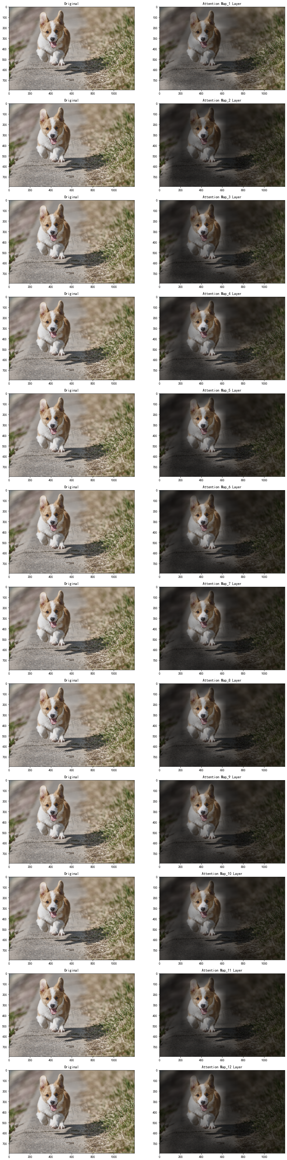
逐层展示attention分布图（同样是每层所有header的attention值求平均），如下：

在cifar10数据集训练模型后，对柯基做分类的结果如下：

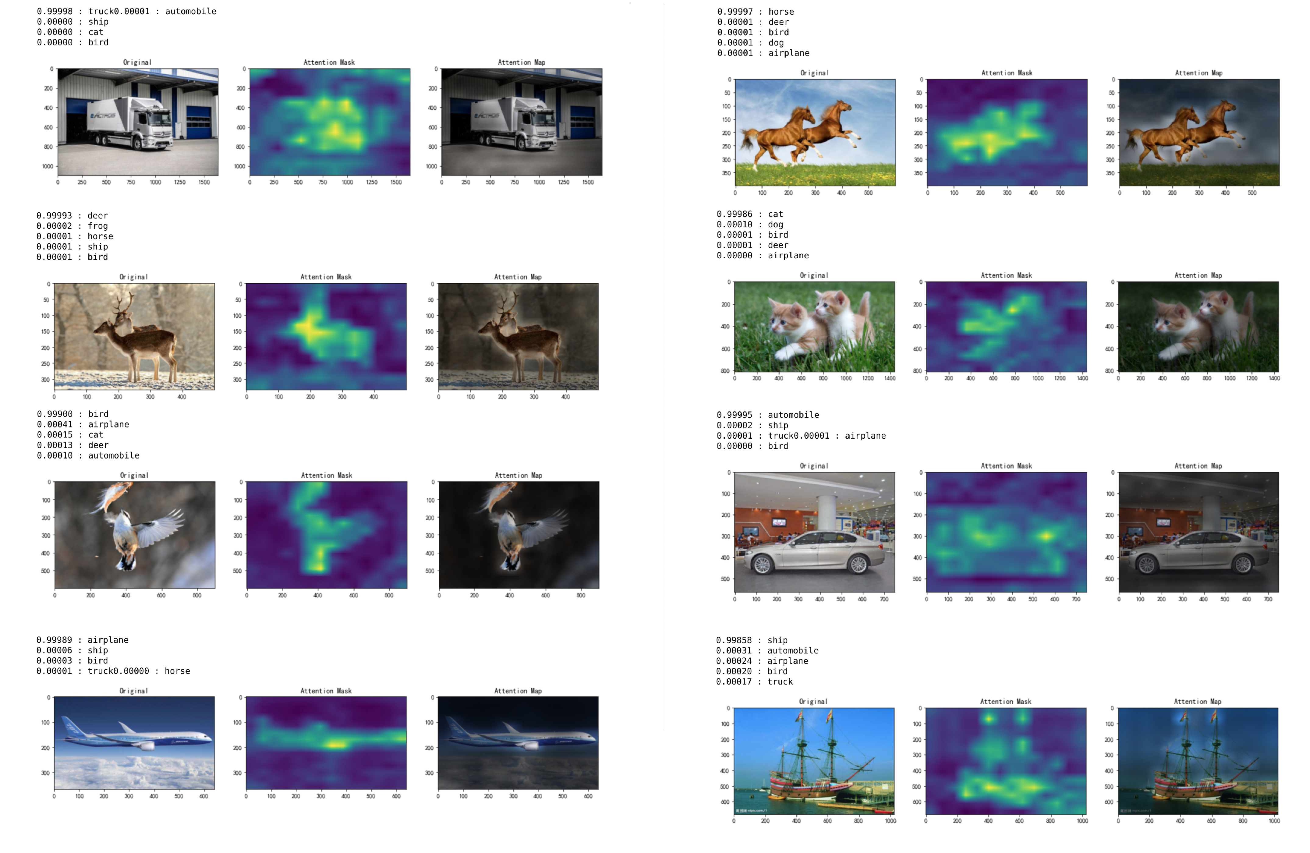
其他例子可视化：

模型训练以cifar10分类问题为例，利用torchvision的datasets模块自动下载和组织训练与测试数据集，并利用transforms模块做样本处理，类似这样：

transform_train = transforms.Compose([
      transforms.RandomResizedCrop(img_size, scale=(0.05, 1.0)),
      transforms.ToTensor(),
      transforms.Normalize(mean=[0.5, 0.5, 0.5], std=[0.5, 0.5, 0.5]),
  ])
transform_test = transforms.Compose([
    transforms.Resize(img_size),
    transforms.ToTensor(),
    transforms.Normalize(mean=[0.5, 0.5, 0.5], std=[0.5, 0.5, 0.5]),
])
trainset = datasets.CIFAR10(root="./data",
                                  train=True,
                                  download=True,
                                  transform=transform_train)
testset = datasets.CIFAR10(root="./data",
                           train=False,
                           download=True,
                           transform=transform_test)

之后以batch方式训练和验证模型，如下：

def train(self):
  """
  training the model
  :return: None
  """

  self.load_model()
  # 加载训练数据和测试数据
  train_loader, test_loader = data_loader(self.config.items.img_size,
                                          self.config.items.train_batch_size,
                                          self.config.items.test_batch_size)
  # 选择一个一阶最优化方法
  if self.config.items.optimizer == 'adam':
      optimizer = torch.optim.Adam(self.model.parameters(),
                                   lr=self.config.items.learning_rate)
  elif self.config.items.optimizer == 'adagrad':
      optimizer = torch.optim.Adagrad(self.model.parameters(),
                                      lr=self.config.items.learning_rate)
  else:
      optimizer = torch.optim.SGD(self.model.parameters(),
                                  lr=self.config.items.learning_rate,
                                  momentum=0.9)

  # 总的迭代步数
  t_total = self.config.items.num_steps
  # 以此步数做学习率分段函数
  warmup_steps = self.config.items.warmup_steps
  # 随着迭代步数增加，调整学习率的策略(cosine法|S)
  #        *
  #       *   *
  #      *      *
  #     *        *
  #    *          *
  #   *            *
  #  *               *
  # *                   *
  # *                       *   *    *
  scheduler = LambdaLR(optimizer=optimizer,
                       lr_lambda=lambda step: float(step) / warmup_steps if step < warmup_steps else 0.5 * (
                               math.cos(math.pi * 0.6 * 2.0 * (step - warmup_steps) / (
                                       t_total - warmup_steps)) + 1.0))

  print("\r\n***** Running training *****")

  # 模型所有参数梯度值初始化为0
  self.model.zero_grad()
  # 计算平均损失
  loss_sum = 0
  loss_count = 0
  # 当前迭代步数
  current_step = 0
  # 当前最佳精度
  current_best_acc = 0

  while True:
      self.model.train()
      # 初始化进度条
      epoch_iterator = tqdm(train_loader,
                            desc="Training Progress [x / x Total Steps] {loss=x.x}",
                            bar_format="{l_bar}{r_bar}",
                            dynamic_ncols=True)

      for step, batch in enumerate(epoch_iterator):
          # 获取一个batch，并把数据发送到相应设备上（如：GPU卡）
          batch = tuple(t.to(self.config.items.device) for t in batch)
          # 特征与标注数据
          features, label = batch
          loss, _ = self.model(features, label)
          # 自动反向传播求梯度
          loss.backward()
          # 全局平均损失
          loss_sum += loss.item()
          loss_count += 1
          # 梯度正则化，缓解过拟合
          torch.nn.utils.clip_grad_norm_(self.model.parameters(), 1)
          # 执行一步最优化方法
          optimizer.step()
          # 执行学习率调整策略
          scheduler.step()
          # 梯度清零
          optimizer.zero_grad()
          # 存储当前迭代步数
          current_step += 1

          epoch_iterator.set_description(
              "Training Progress [%d / %d Total Steps] {loss=%2.5f}" % (
                  current_step, t_total, loss_sum / loss_count)
          )

          self.writer.add_scalar("train/loss", scalar_value=loss_sum / loss_count, global_step=current_step)
          self.writer.add_scalar("train/lr", scalar_value=scheduler.get_last_lr()[0], global_step=current_step)

          # 每迭代若干步后做测试集验证
          if current_step % self.config.items.test_epoch == 0:
              accuracy = self.test(test_loader, current_step)
              # 测试集上表现好的模型被存储，并更新当前最佳精度
              if current_best_acc < accuracy:
                  self.save_model()
                  current_best_acc = accuracy
              # 接着训练
              self.model.train()

          if current_step % t_total == 0:
              break
      loss_sum = 0
      loss_count = 0
      if current_step % t_total == 0:
          break

  self.writer.close()
  print("Best Accuracy: \t%f" % current_best_acc)
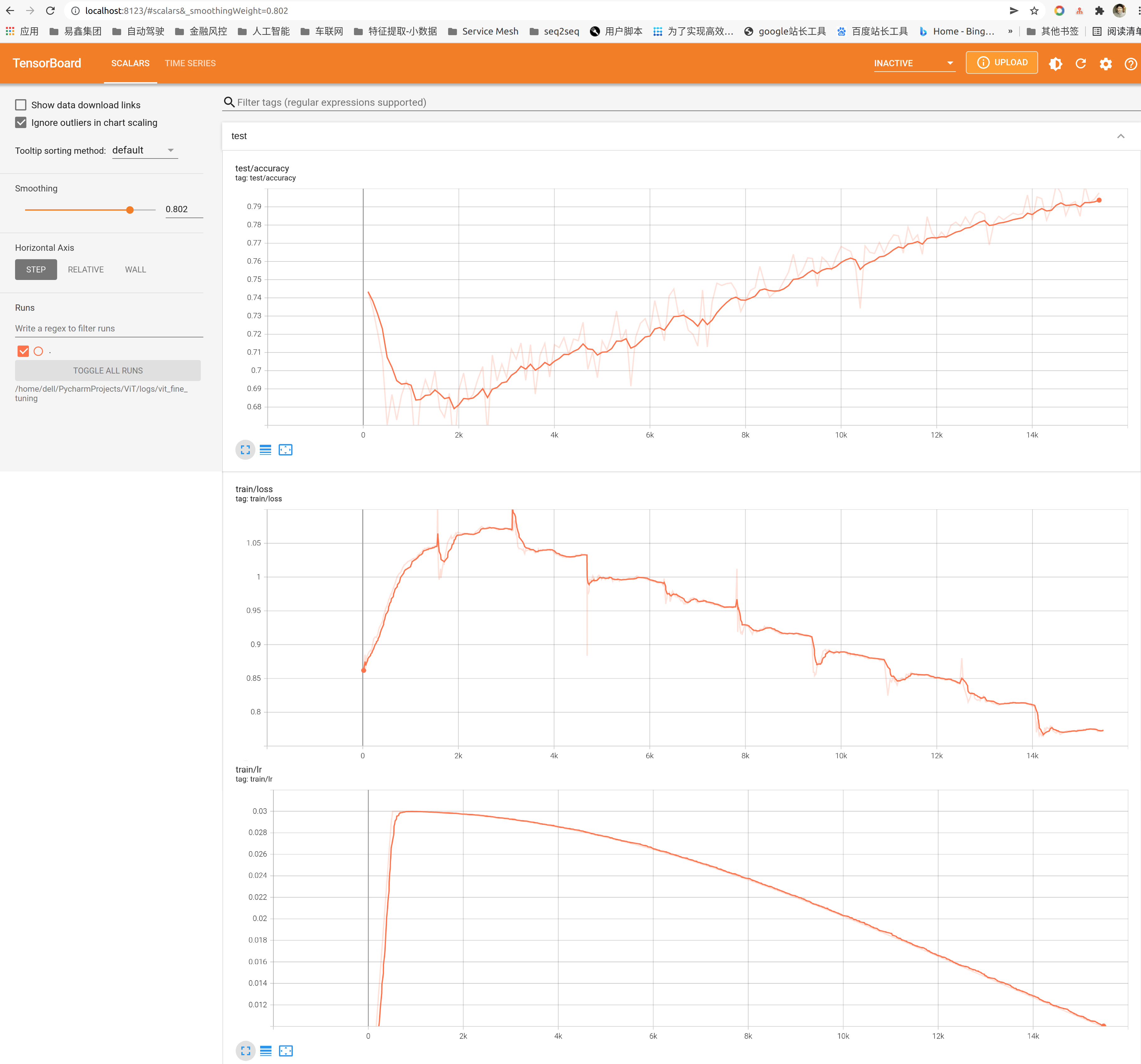
  print("***** End Training *****")

需要注意，为了提升训练效果，学习率采用分段函数调整，训练前期猛一点，采用线性增长，过了一定阈值后逐步平缓，采用cosine下降。另外将训练的过程数据写入日志，可以利用tensorboard可视化的查看训练过程，执行命令诸如：

1	tensorboard --logdir=*** --port 8123

可以在浏览器查看，如：

以上是对最初transformer机制被应用于CV的简单介绍和代码实践，完整代码在这里。

3、小结

ViT有两个很关键的点：

采用self-attention机制捕获序列中元素的长依赖（long term dependencies）；
利用在大规模数据集（如：ImageNet）上训练的模型作为预训练模型（pre-training）会有好的效果，反过来说，如果数据集不够大，预训练模型的泛化性会比较差。

实践证明得益于Transformer这种结构带来的优点，使得它有比较大的潜力，也成为了后续CV的重点研究领域，期待未来有更好的表现。

10.2 DeiT

初版ViT有一个很大的问题是：要想模型效果好，训练数据集要很大，不管是数据集获取难度还是训练速度都受限，FB在《Training data-efficient image transformers & distillation through attention》一文提出一种解决该问题的方法，

优点是：只是用ImageNet这样的公开数据集做训练，纯Transformer结构，对初版ViT只做了比较小的改动，由于使用蒸馏机制，使得训练速度大大提升，单机8卡训练了3天，DeiT-B 384在只使用88M参数量规模下达到了Top 1 Accuracy 85.2% 的效果，Image Classification on ImageNet 榜单排名84（截止2022.1.6）。

缺点是：需要一个预训练好的CNN模型当teacher，所以显然最终效果受teacher影响极大。

1、模型结构 相比初版ViT，它主要在Embedding层增加了一个类似class token的distillation token，前者表征了对真实标签的全局隐语义概括，后者表征了对teacher模型的预测标签的全局隐语义概括。具体结构如下：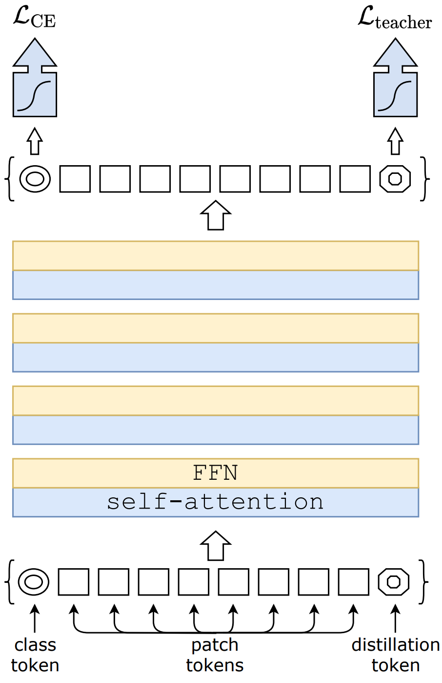

损失函数方面，初版ViT采用预测值与真实标签的交叉熵损失，DeiT除此之外增加了蒸馏损失，即预测值与teacher模型的预测标签的交叉熵损失，细节如下：

软蒸馏（Soft Distillation） \[ \mathcal{L}_{global}=(1-\lambda)\mathcal{L}_{CE}(\psi(Z_s),y)+\lambda \tau ^2KL(\psi(Z_s/\tau),\psi(Z_t/\tau)) \] 其中，$y$为真实标签，$\psi$为softmax函数，$\tau$为蒸馏参数，$\lambda$ 是用来平衡交叉熵损失和e Kullback–Leibler divergence 损失的，$\mathcal{L}_{CE}$为交叉熵损失。
硬蒸馏（Hard-label Distillation） \[ \mathcal{L}_{global}^{hardDistill}=\frac{1}{2}\mathcal{L}_{CE}(\psi(Z_s),y)+\frac{1}{2}\mathcal{L}_{CE}(\psi(Z_s),y_t) \] 其中，$ y_t = argmax_cZ_t(c) $是把teacher的预测标签当做真实标签。一个有趣的现象是：class token和distillation token会朝不同方向收敛，且随着迭代次数和层数，这两个向量的cosine相似度会越来越接近（但不会相等）。

2、实验结论

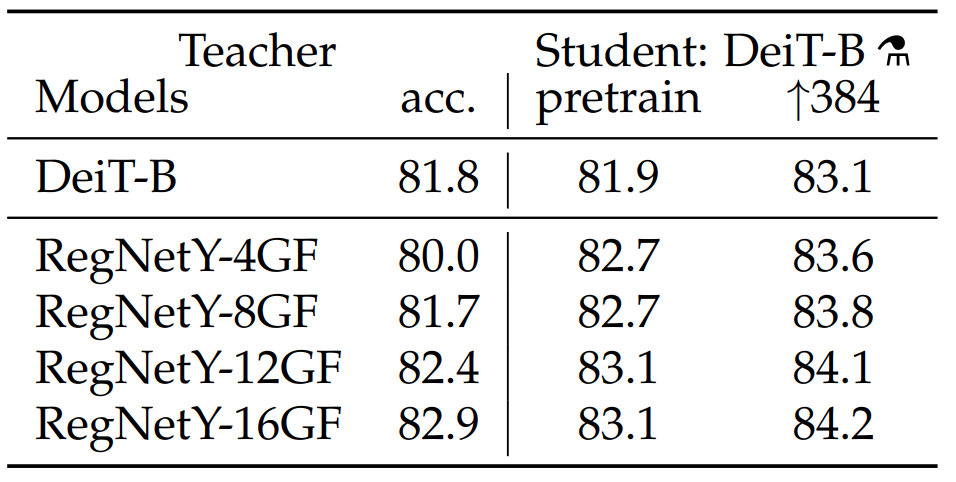
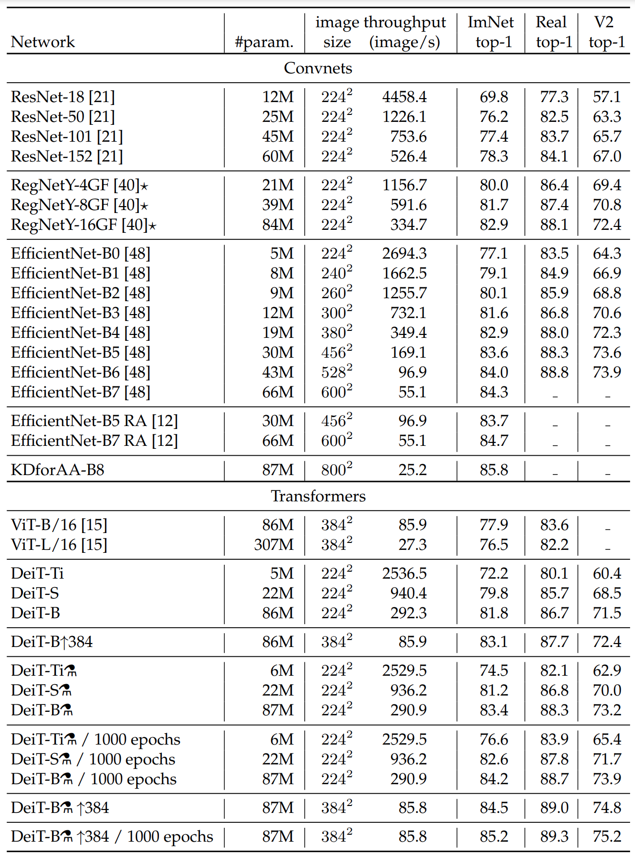
不同的DeiT结构及效果如下：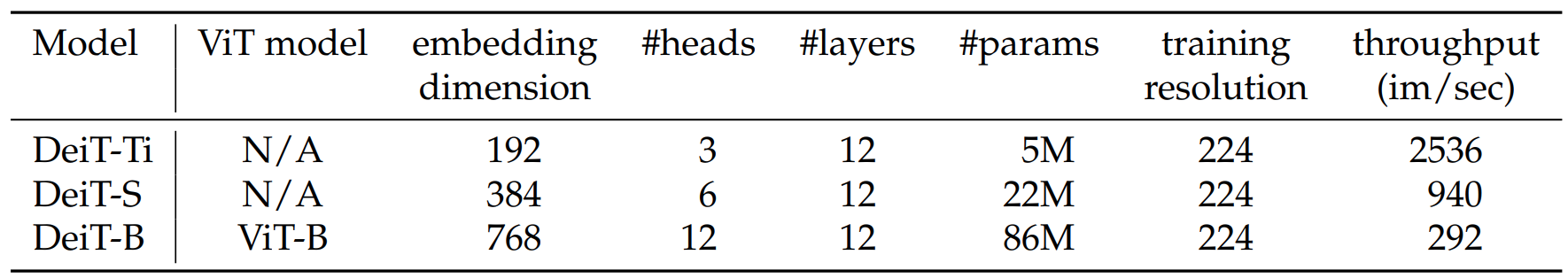

CNN类模型作为teacher比transformer类模型效果更好，原因可能是transformer通过蒸馏继承了归纳偏置导致，具体解释可以看这篇论文。
上图中：384代表fine-tuning得到的模型使用了分辨率为384×384图像做训练，⚗代表蒸馏后得到的模型。
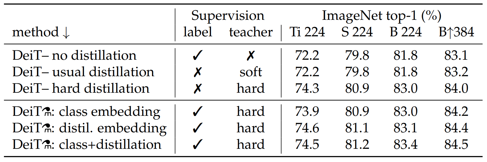
硬蒸馏效果好于软蒸馏和不蒸馏，同时使用class token和distillation token效果好于只是用其中一个。
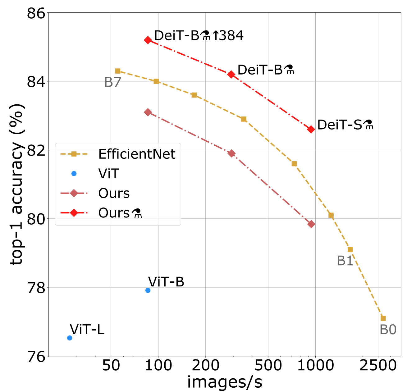
效率与精度对比
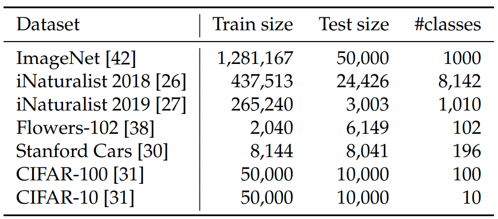
只使用从ImageNet数据集训练出来的模型作为预训练模型，各个模型迁移到不同任务的效果对比如下，DeiT更胜一筹。数据集使用：
效果对比：
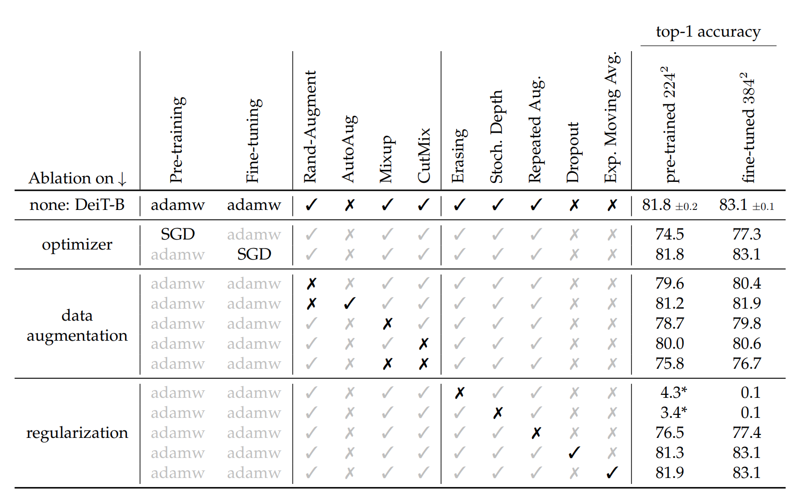
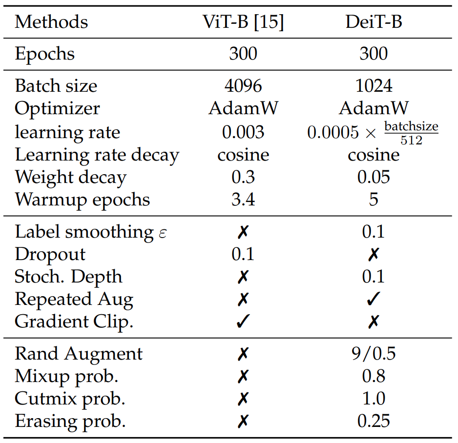
相对来说Transformers模型对优化器的参数更敏感

3、代码实践

继承之前的VisionTransformer实现并增加distillation token向量：

class DistillationEmbeddings(Embeddings):
    def __init__(self, image_hw, dim_of_model, channels=3, patch_size=16, dropout=0.1):
        super().__init__(image_hw, dim_of_model, channels, patch_size, dropout)

        self.distillation_token = nn.Parameter(torch.zeros(1, 1, dim_of_model))

    def forward(self, x):
        batch_size = x.shape[0]
        cls_tokens = self.class_token.expand(batch_size, -1, -1)
        dis_tokens = self.distillation_token.expand(batch_size, -1, -1)

        x = self.patch_embeddings(x)
        x = x.flatten(2)
        x = x.transpose(-1, -2)
        x = torch.cat((cls_tokens, x), dim=1)

        embeddings = x + self.position_embeddings
        embeddings = torch.cat((embeddings, dis_tokens), dim=1)
        embeddings = self.dropout(embeddings)
        return embeddings

class DistillationTransformerEncoder(TransformerEncoder):
    def __init__(self, num_of_heads, dim_of_model, dim_of_mlp, num_layers,
                 image_hw, channels=3, patch_size=16,
                 em_dropout=0.1, atten_dropout=0.1, mlp_dropout=0.1):
        super().__init__(num_of_heads, dim_of_model, dim_of_mlp, num_layers,
                         image_hw, channels, patch_size,
                         em_dropout, atten_dropout, mlp_dropout)

        self.embeddings = DistillationEmbeddings(image_hw, dim_of_model, channels, patch_size, em_dropout)
        self.transformer_encoder = Encoder(num_of_heads, dim_of_model, dim_of_mlp, num_layers, atten_dropout,
                                           mlp_dropout)

class DistillationVisionTransformer(VisionTransformer):
    def __init__(self, num_of_heads, dim_of_model, dim_of_mlp, num_layers,
                 image_hw=(224, 224), channels=3, patch_size=16,
                 em_dropout=0.1, atten_dropout=0.1, mlp_dropout=0.1, num_classes=10,
                 teacher=None, is_hard=False, temperature=3.0, balancing=0.1):

        super().__init__(num_of_heads, dim_of_model, dim_of_mlp, num_layers,
                         image_hw, channels, patch_size,
                         em_dropout, atten_dropout, mlp_dropout, num_classes)

        self.transformer = DistillationTransformerEncoder(self.num_of_heads, self.dim_of_model, self.dim_of_mlp,
                                                          self.num_layers,
                                                          self.image_hw, self.channels, self.patch_size,
                                                          self.em_dropout, self.atten_dropout, self.mlp_dropout)
        self.teacher = teacher
        self.is_hard = is_hard
        self.temperature = temperature
        self.balancing = balancing

    def forward(self, x, labels=None):
        encoded, attention_weights = self.transformer(x)
        student_logits = self.vit_head(encoded[:, 0])
        with torch.no_grad():
            teacher_logits = self.teacher(x)

        if labels is not None:
            if not self.is_hard:
                loss = soft_distillation(teacher_logits, student_logits,
                                         self.temperature, self.balancing, labels, self.num_classes)
            else:
                loss = hard_distillation(teacher_logits, student_logits,
                                         self.balancing, labels, self.num_classes)

            return loss, student_logits
        else:
            return student_logits, attention_weights

import torch
import torch.nn.functional as F


def soft_distillation(teacher_logits, student_logits, temperature, balancing, labels, num_classes):
    loss_function = torch.nn.CrossEntropyLoss()
    kl_loss = F.kl_div(
        F.log_softmax(student_logits / temperature, dim=-1),
        F.softmax(teacher_logits / temperature, dim=-1).detach(),
        reduction='batchmean')

    kl_loss *= (balancing * temperature ** 2)

    student_loss = loss_function(student_logits.view(-1, num_classes), labels.view(-1))
    return (1 - balancing) * student_loss + kl_loss


def hard_distillation(teacher_logits, student_logits, balancing, labels, num_classes):
    loss_function = torch.nn.CrossEntropyLoss()
    teacher_labels = teacher_logits.argmax(dim=-1)
    teacher_loss = loss_function(teacher_logits.view(-1, num_classes), teacher_labels.view(-1))
    student_loss = loss_function(student_logits.view(-1, num_classes), labels.view(-1))

    return (1 - balancing) * student_loss + balancing * teacher_loss

完整代码在这里。

总结来说，DeiT的贡献主要是能够只在ImageNet数据集上训练出一个纯Transformer模型，并利用蒸馏技术可以使得Transformer在较小的数据集上就能达到较好的效果，其缺点也很明显，依赖一个CNN模型作为teacher且Transformer的效果依赖teacher的效果。

业精于勤，荒于嬉；行成于思，毁于随。

机器学习与人工智能技术分享-第十章-Vision Transformers (ViT)

10. Vision Transformers

10.1 初版Vit

10.2 DeiT