本章对机器学习在计算机视觉尤其是目标检测与识别方面的各种代表性模型和算法做了原理介绍和效果展示。
8. 目标检测与识别
目标检测的发展历程大致如下: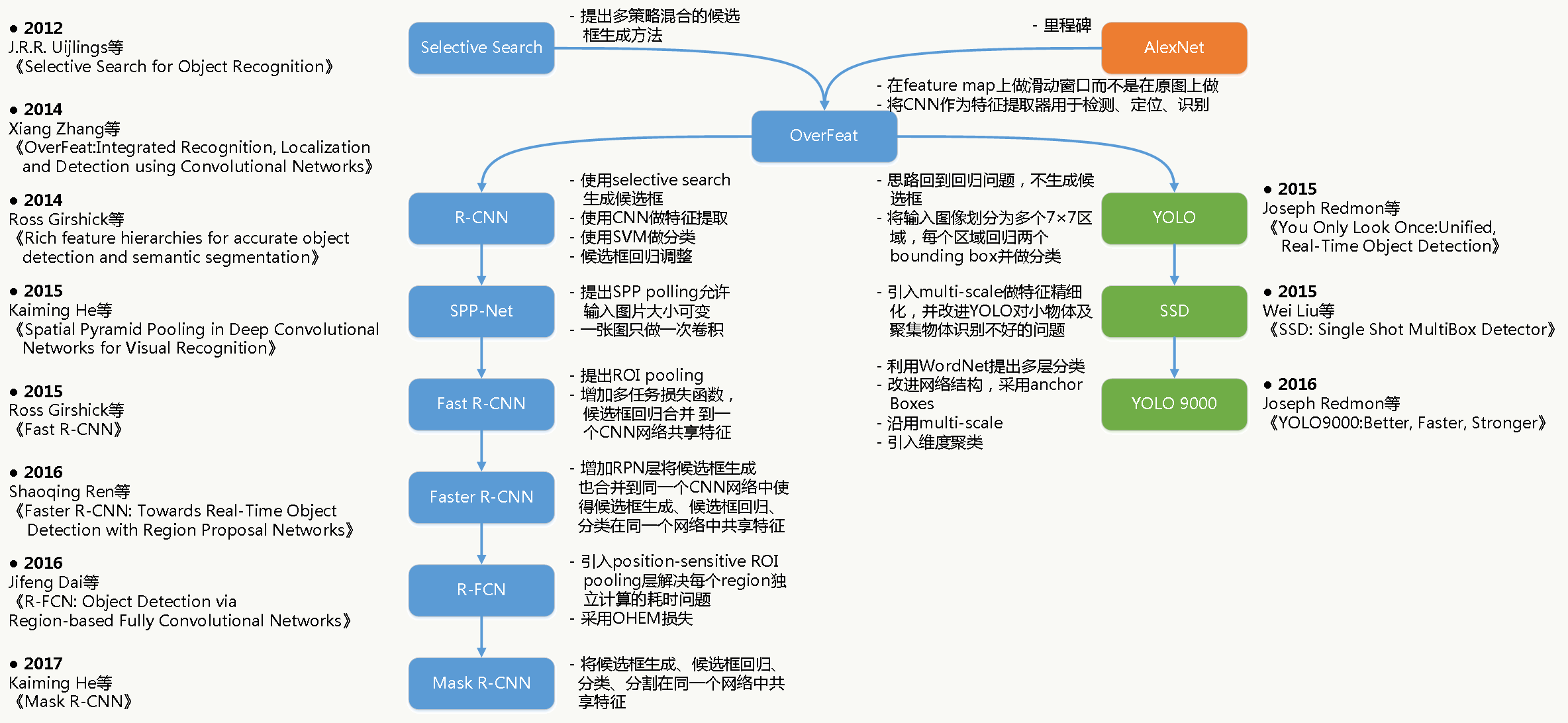
8.1 Selective Search
对于目标识别任务,比如判断一张图片中有没有车、是什么车,一般需要解决两个问题:目标检测、目标识别。而目标检测任务中通常需要先通过某种方法做图像分割,事先得到候选框;直观的做法是:给定窗口,对整张图片滑动扫描,结束后改变窗口大小重复上面步骤,缺点很明显:重复劳动耗费资源、精度和质量不高等等。 针对上面的问题,一种解决方案是借鉴启发式搜索的方法,充分利用人类的先验知识。J.R.R. Uijlings在《Selective Search for Object Recoginition》提出一种方法:基于数据驱动,与具体类别无关的多种策略融合的启发式生成方法。图片包含各种丰富信息,例如:大小、形状、颜色、纹理、物体重叠关系等,如果只使用一种信息往往不能解决大部分问题,例如: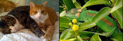
左边的两只猫可以通过颜色区别而不是通过纹理,右面的变色龙却只能通过纹理区别而不是颜色。
8.1.1 启发式生成设计准则
所以概括来说:
- 能够捕捉到各种尺度物体,大的、小的、边界清楚的、边界模糊的等等; 多尺度的例子:
- 策略多样性,采用多样的策略集合共同作用;
- 计算快速,由于生成候选框只是检测第一步,所以计算上它决不能成为瓶颈。
8.1.2 Selective Search
基于以上准则设计Selective Search算法:
采用层次分组算法解决尺度问题
引入图像分割中的自下而上分组思想,由于整个过程是层次的,在将整个图合并成一个大的区域的过程中会输出不同尺度的多个子区域。整个过程如下:
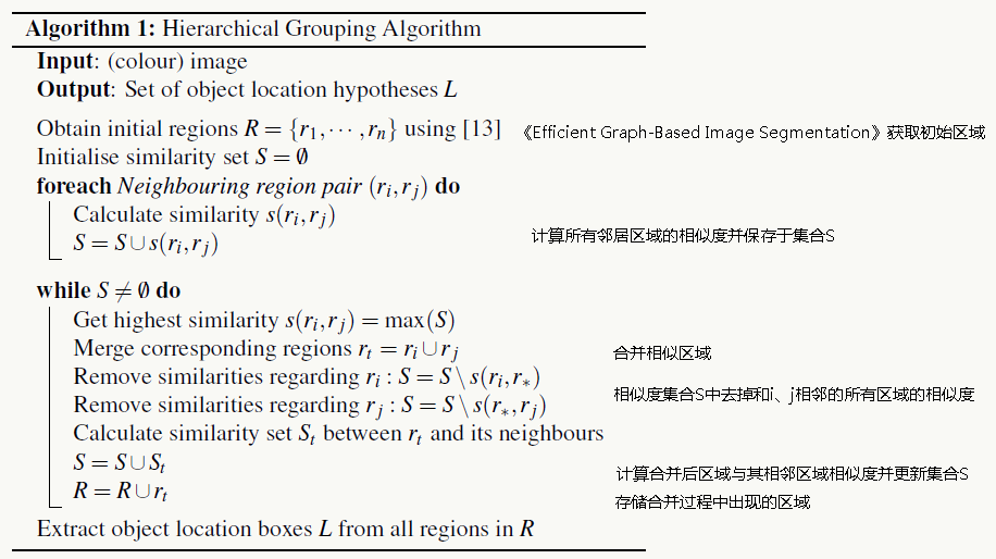
1、利用《Efficient Graph-Based Image Segmentation》(基本思想:将图像中每个像素表示为图上的一个节点,用于连接不同节点的无向边都有一个权重,这个权重表示两个节点之间的不相似度,通过贪心算法利用最小生成树做图像分割)生成初始候选区域;
2、采用贪心算法合并区域,计算任意两个领域的相似度,把达到阈值的合并,再计算新区域和其所有领域的相似度,循环迭代,直到整个图变成了一个区域,算法如下:
![]()
多样化策略
三个方面:使用多种颜色空间、使用多种相似度计算方法、搜索起始区域不固定。
1、颜色空间有很多种:RGB、HSV、Lab等等,不是论文重点;
2、相似度衡量算法,结合了4重策略:
颜色相似度
以RGB为例,使用L1-norm归一化每个图像通道的色彩直方图(bins=25),每个区域被表示为25×3维向量:\(C_i=\{c_i^1,...,c_i^n\}\); 颜色相似度定义为: \[S_{color}(r_i,r_j)=\sum_{k=1}^nmin(c_i^k,c_j^k)\] 区域合并后对新的区域计算其色彩直方图: \[C_t=\frac{size(r_i)×C_i+size(r_j)×C_j}{size(r_i)+size(r_j)}\] 新区域的大小为:\(size(r_t)=size(r_i)+size(r_j)\)
纹理相似度
使用快速生成的类SIFT特征,对每个颜色通道在8个方向上应用方差为1的高斯滤波器,对每个颜色通道的每个方向提取bins=10的直方图,所以整个纹理向量维度为:3×8×10=240,表示为:\(T_i=\{t_i^1,...,t_i^n\}\); 纹理相似度定义为: \[S_{texture}(r_i,r_j)=\sum_{k=1}^nmin(t_i^k,t_j^k)\]
大小相似度
该策略希望小的区域能尽早合并,让合并操作比较平滑,防止出现某个大区域逐步吞并其他小区域的情况。相似度定义为: \[S_{size}=1-\frac{size(r_i)+size(r_j)}{size(im)}\] 其中\(size(im)\)为图像包含像素点数目。
区域规则度相似度
能够框住合并后的两个区域的矩形大小越小说明两个区域的合并越规则,如: 区域规则度相似度定义为: \[S_{fill}=1-\frac{size(BB_{i,j})-size(r_i)-size(r_j)}{size(im)}\]
最终相似度为所有策略加权和,文中采用等权方式: \[S_{r_i,r_j}=\alpha_1\cdot S_{color}(r_i,r_j)+\alpha_2\cdot S_{texture}(r_i,r_j)+\alpha_3\cdot S_{size}(r_i,r_j)+\alpha_4\cdot S_{fill}(r_i,r_j)\]
8.1.3 使用Selective Search做目标识别
训练过程包含:提取候选框、提取特征、生成正负样本、训练模型,图示如下: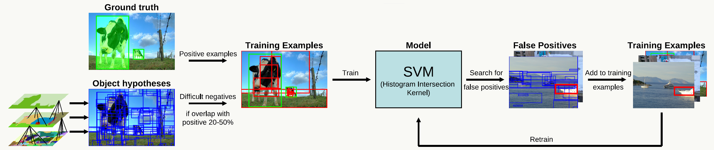
早期图像特征提取往往是各种HOG特征或BoW特征,现在CNN特征几乎一统天下。 检测定位效果评价采用Average Best Overlap(ABO)和Mean Average Best Overlap(MABO): \[ ABO=\frac{1}{|G^c|}\sum_{g_i^c\in G^c}max_{I_j\in L} Overlap(g_i^c,l_j) \] 其中:\(c\)为类别标注、\(g_i^c\)为类别\(c\)下的ground truth,\(L\)为通过Selective Search生成的候选框。 \[ MABO=\frac{1}{|C|}\sum_{i=1}^n ABO(C_i) \]
8.1.4 代码实践
参见AlpacaDB。
- selectivesearch.py
1
2
3
4
5
6
7
8
9
10
11
12
13
14
15
16
17
18
19
20
21
22
23
24
25
26
27
28
29
30
31
32
33
34
35
36
37
38
39
40
41
42
43
44
45
46
47
48
49
50
51
52
53
54
55
56
57
58
59
60
61
62
63
64
65
66
67
68
69
70
71
72
73
74
75
76
77
78
79
80
81
82
83
84
85
86
87
88
89
90
91
92
93
94
95
96
97
98
99
100
101
102
103
104
105
106
107
108
109
110
111
112
113
114
115
116
117
118
119
120
121
122
123
124
125
126
127
128
129
130
131
132
133
134
135
136
137
138
139
140
141
142
143
144
145
146
147
148
149
150
151
152
153
154
155
156
157
158
159
160
161
162
163
164
165
166
167
168
169
170
171
172
173
174
175
176
177
178
179
180
181
182
183
184
185
186
187
188
189
190
191
192
193
194
195
196
197
198
199
200
201
202
203
204
205
206
207
208
209
210
211
212
213
214
215
216
217
218
219
220
221
222
223
224
225
226
227
228
229
230
231
232
233
234
235
236
237
238
239
240
241
242
243
244
245
246
247
248
249
250
251
252
253
254
255
256
257
258
259
260
261
262
263
264
265
266
267
268
269
270
271
272
273
274
275
276
277
278
279
280
281
282
283
284
285
286
287
288
289
290
291
292
293
294
295
296
297
298
299
300
301
302
303
304
305
306
307
308
309
# -*- coding: utf-8 -*-
import skimage.io
import skimage.feature
import skimage.color
import skimage.transform
import skimage.util
import skimage.segmentation
import numpy
# "Selective Search for Object Recognition" by J.R.R. Uijlings et al.
#
# - Modified version with LBP extractor for texture vectorization
def _generate_segments(im_orig, scale, sigma, min_size):
"""
segment smallest regions by the algorithm of Felzenswalb and
Huttenlocher
"""
# open the Image
im_mask = skimage.segmentation.felzenszwalb(
skimage.util.img_as_float(im_orig), scale=scale, sigma=sigma,
min_size=min_size)
# merge mask channel to the image as a 4th channel
im_orig = numpy.append(
im_orig, numpy.zeros(im_orig.shape[:2])[:, :, numpy.newaxis], axis=2)
im_orig[:, :, 3] = im_mask
return im_orig
def _sim_colour(r1, r2):
"""
calculate the sum of histogram intersection of colour
"""
return sum([min(a, b) for a, b in zip(r1["hist_c"], r2["hist_c"])])
def _sim_texture(r1, r2):
"""
calculate the sum of histogram intersection of texture
"""
return sum([min(a, b) for a, b in zip(r1["hist_t"], r2["hist_t"])])
def _sim_size(r1, r2, imsize):
"""
calculate the size similarity over the image
"""
return 1.0 - (r1["size"] + r2["size"]) / imsize
def _sim_fill(r1, r2, imsize):
"""
calculate the fill similarity over the image
"""
bbsize = (
(max(r1["max_x"], r2["max_x"]) - min(r1["min_x"], r2["min_x"]))
* (max(r1["max_y"], r2["max_y"]) - min(r1["min_y"], r2["min_y"]))
)
return 1.0 - (bbsize - r1["size"] - r2["size"]) / imsize
def _calc_sim(r1, r2, imsize):
return (_sim_colour(r1, r2) + _sim_texture(r1, r2)
+ _sim_size(r1, r2, imsize) + _sim_fill(r1, r2, imsize))
def _calc_colour_hist(img):
"""
calculate colour histogram for each region
the size of output histogram will be BINS * COLOUR_CHANNELS(3)
number of bins is 25 as same as [uijlings_ijcv2013_draft.pdf]
extract HSV
"""
BINS = 25
hist = numpy.array([])
for colour_channel in (0, 1, 2):
# extracting one colour channel
c = img[:, colour_channel]
# calculate histogram for each colour and join to the result
hist = numpy.concatenate(
[hist] + [numpy.histogram(c, BINS, (0.0, 255.0))[0]])
# L1 normalize
hist = hist / len(img)
return hist
def _calc_texture_gradient(img):
"""
calculate texture gradient for entire image
The original SelectiveSearch algorithm proposed Gaussian derivative
for 8 orientations, but we use LBP instead.
output will be [height(*)][width(*)]
"""
ret = numpy.zeros((img.shape[0], img.shape[1], img.shape[2]))
for colour_channel in (0, 1, 2):
ret[:, :, colour_channel] = skimage.feature.local_binary_pattern(
img[:, :, colour_channel], 8, 1.0)
return ret
def _calc_texture_hist(img):
"""
calculate texture histogram for each region
calculate the histogram of gradient for each colours
the size of output histogram will be
BINS * ORIENTATIONS * COLOUR_CHANNELS(3)
"""
BINS = 10
hist = numpy.array([])
for colour_channel in (0, 1, 2):
# mask by the colour channel
fd = img[:, colour_channel]
# calculate histogram for each orientation and concatenate them all
# and join to the result
hist = numpy.concatenate(
[hist] + [numpy.histogram(fd, BINS, (0.0, 1.0))[0]])
# L1 Normalize
hist = hist / len(img)
return hist
def _extract_regions(img):
R = {}
# get hsv image
hsv = skimage.color.rgb2hsv(img[:, :, :3])
# pass 1: count pixel positions
for y, i in enumerate(img):
for x, (r, g, b, l) in enumerate(i):
# initialize a new region
if l not in R:
R[l] = {
"min_x": 0xffff, "min_y": 0xffff,
"max_x": 0, "max_y": 0, "labels": [l]}
# bounding box
if R[l]["min_x"] > x:
R[l]["min_x"] = x
if R[l]["min_y"] > y:
R[l]["min_y"] = y
if R[l]["max_x"] < x:
R[l]["max_x"] = x
if R[l]["max_y"] < y:
R[l]["max_y"] = y
# pass 2: calculate texture gradient
tex_grad = _calc_texture_gradient(img)
# pass 3: calculate colour histogram of each region
for k, v in R.items():
# colour histogram
masked_pixels = hsv[:, :, :][img[:, :, 3] == k]
R[k]["size"] = len(masked_pixels / 4)
R[k]["hist_c"] = _calc_colour_hist(masked_pixels)
# texture histogram
R[k]["hist_t"] = _calc_texture_hist(tex_grad[:, :][img[:, :, 3] == k])
return R
def _extract_neighbours(regions):
def intersect(a, b):
if (a["min_x"] < b["min_x"] < a["max_x"]
and a["min_y"] < b["min_y"] < a["max_y"]) or (
a["min_x"] < b["max_x"] < a["max_x"]
and a["min_y"] < b["max_y"] < a["max_y"]) or (
a["min_x"] < b["min_x"] < a["max_x"]
and a["min_y"] < b["max_y"] < a["max_y"]) or (
a["min_x"] < b["max_x"] < a["max_x"]
and a["min_y"] < b["min_y"] < a["max_y"]):
return True
return False
R = regions.items()
neighbours = []
for cur, a in enumerate(R[:-1]):
for b in R[cur + 1:]:
if intersect(a[1], b[1]):
neighbours.append((a, b))
return neighbours
def _merge_regions(r1, r2):
new_size = r1["size"] + r2["size"]
rt = {
"min_x": min(r1["min_x"], r2["min_x"]),
"min_y": min(r1["min_y"], r2["min_y"]),
"max_x": max(r1["max_x"], r2["max_x"]),
"max_y": max(r1["max_y"], r2["max_y"]),
"size": new_size,
"hist_c": (
r1["hist_c"] * r1["size"] + r2["hist_c"] * r2["size"]) / new_size,
"hist_t": (
r1["hist_t"] * r1["size"] + r2["hist_t"] * r2["size"]) / new_size,
"labels": r1["labels"] + r2["labels"]
}
return rt
def selective_search(
im_orig, scale=1.0, sigma=0.8, min_size=50):
'''Selective Search
Parameters
----------
im_orig : ndarray
Input image
scale : int
Free parameter. Higher means larger clusters in felzenszwalb segmentation.
sigma : float
Width of Gaussian kernel for felzenszwalb segmentation.
min_size : int
Minimum component size for felzenszwalb segmentation.
Returns
-------
img : ndarray
image with region label
region label is stored in the 4th value of each pixel [r,g,b,(region)]
regions : array of dict
[
{
'rect': (left, top, right, bottom),
'labels': [...]
},
...
]
'''
assert im_orig.shape[2] == 3, "3ch image is expected"
# load image and get smallest regions
# region label is stored in the 4th value of each pixel [r,g,b,(region)]
img = _generate_segments(im_orig, scale, sigma, min_size)
if img is None:
return None, {}
imsize = img.shape[0] * img.shape[1]
R = _extract_regions(img)
# extract neighbouring information
neighbours = _extract_neighbours(R)
# calculate initial similarities
S = {}
for (ai, ar), (bi, br) in neighbours:
S[(ai, bi)] = _calc_sim(ar, br, imsize)
# hierarchal search
while S != {}:
# get highest similarity
i, j = sorted(S.items(), cmp=lambda a, b: cmp(a[1], b[1]))[-1][0]
# merge corresponding regions
t = max(R.keys()) + 1.0
R[t] = _merge_regions(R[i], R[j])
# mark similarities for regions to be removed
key_to_delete = []
for k, v in S.items():
if (i in k) or (j in k):
key_to_delete.append(k)
# remove old similarities of related regions
for k in key_to_delete:
del S[k]
# calculate similarity set with the new region
for k in filter(lambda a: a != (i, j), key_to_delete):
n = k[1] if k[0] in (i, j) else k[0]
S[(t, n)] = _calc_sim(R[t], R[n], imsize)
regions = []
for k, r in R.items():
regions.append({
'rect': (
r['min_x'], r['min_y'],
r['max_x'] - r['min_x'], r['max_y'] - r['min_y']),
'size': r['size'],
'labels': r['labels']
})
return img, regions - example.py
1
2
3
4
5
6
7
8
9
10
11
12
13
14
15
16
17
18
19
20
21
22
23
24
25
26
27
28
29
30
31
32
33
34
35
36
37
38
39
40
41
42
43
44
45
46
47
48
49
50
51
# -*- coding: utf-8 -*-
import matplotlib
matplotlib.use("Agg")
import matplotlib.pyplot as plt
import skimage.data
import skimage.io
from skimage.io import use_plugin,imread
import matplotlib.patches as mpatches
from matplotlib.pyplot import savefig
import selectivesearch
def main():
# loading astronaut image
#img = skimage.data.astronaut()
use_plugin('pil')
img = imread('car.jpg', as_grey=False)
# perform selective search
img_lbl, regions = selectivesearch.selective_search(
img, scale=500, sigma=0.9, min_size=10)
candidates = set()
for r in regions:
# excluding same rectangle (with different segments)
if r['rect'] in candidates:
continue
# excluding regions smaller than 2000 pixels
if r['size'] < 2000:
continue
# distorted rects
x, y, w, h = r['rect']
if w / h > 1.2 or h / w > 1.2:
continue
candidates.add(r['rect'])
# draw rectangles on the original image
plt.figure()
fig, ax = plt.subplots(ncols=1, nrows=1, figsize=(6, 6))
ax.imshow(img)
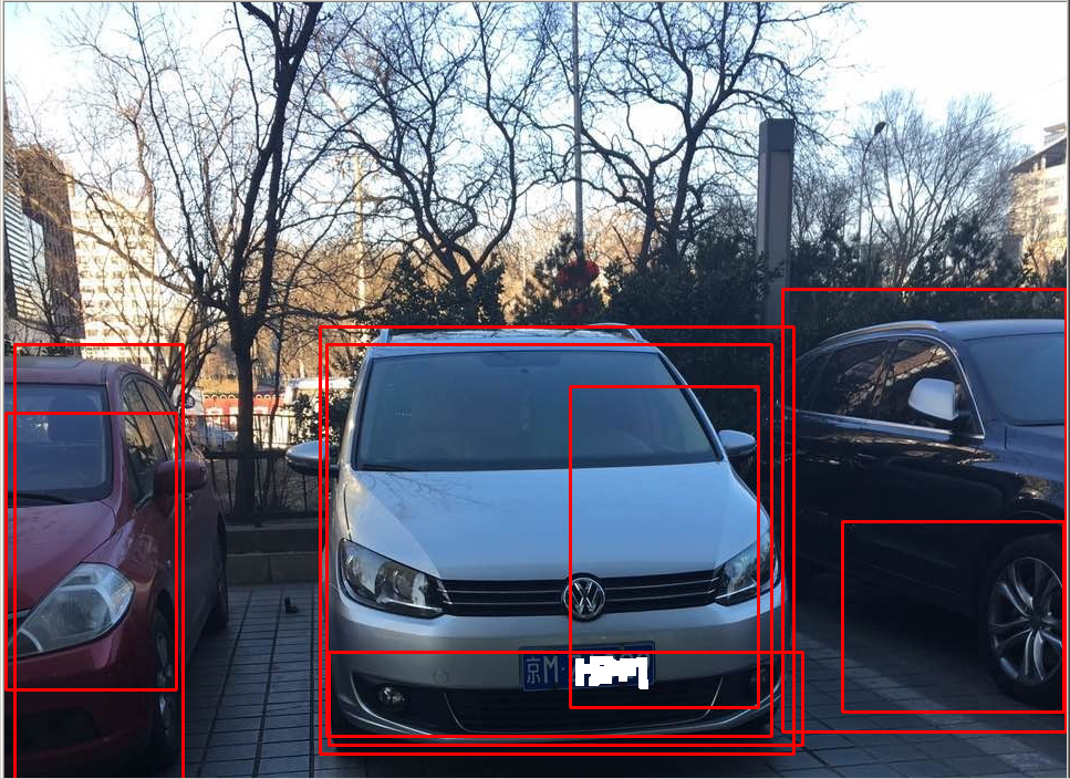
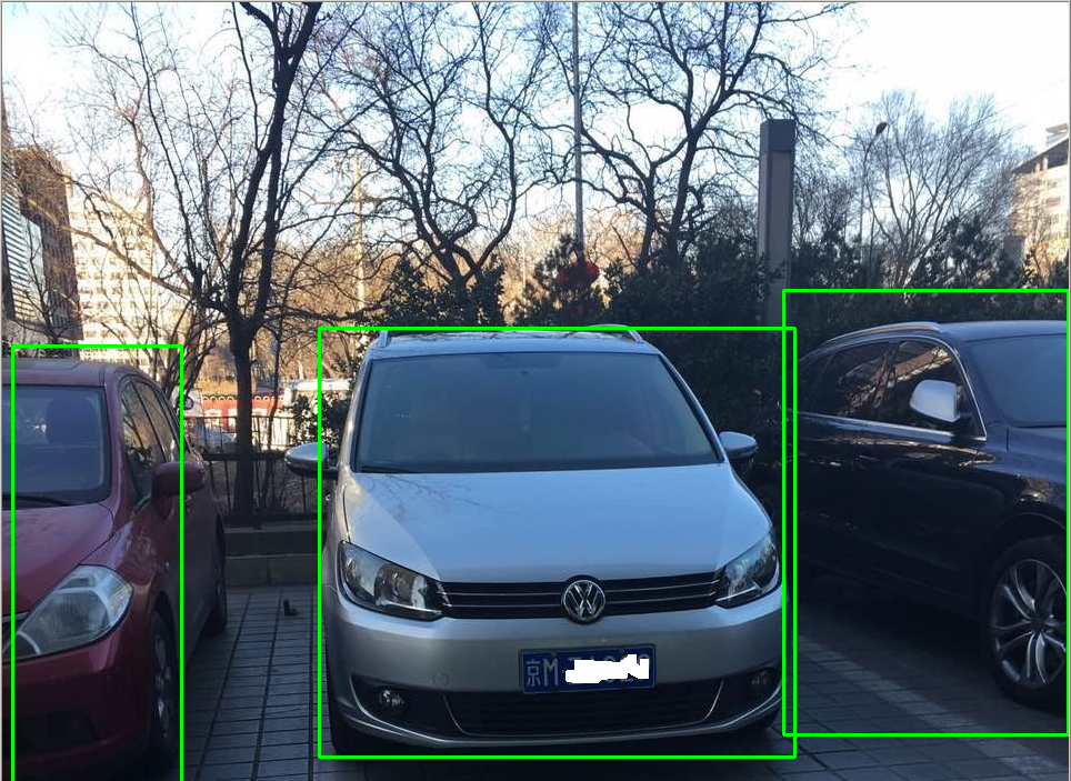
for x, y, w, h in candidates:
print x, y, w, h
rect = mpatches.Rectangle(
(x, y), w, h, fill=False, edgecolor='red', linewidth=1)
ax.add_patch(rect)
#plt.show()
savefig('MyFig.jpg')
if __name__ == "__main__":
main()

8.2 OverFeat
计算机视觉有三大任务:分类(识别)、定位、检测,从左到右每个任务是下个任务的子任务,所以难度递增。OverFeat是2014年《OverFeat:Integrated Recognition, Localization and Detection using Convolutional Networks》中提出的一个基于卷积神经网络的特征提取框架,论文的最大亮点在于通过一个统一的框架去解决图像分类、定位、检测问题,并提出feature map上的一个点可以还原并对应到原图的一个区域,于是一些在原图上的操作可以转到在feature map上做,这点对以后的检测算法有较深远的影响。它在ImageNet 2013的task 3定位任务中获得第一,在检测和分类任务中也有不错的表现。
8.2.1 OverFeat分类任务
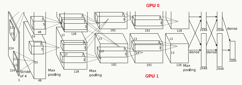
文中借鉴了AlexNet的结构,并做了些结构改进和提高了线上inference效率,结构如下: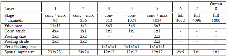
相对AlexNet,网络结构几乎一样,区别在于:
去掉了LRN层,不做额外归一化操作
使用区域非重叠pooling
前两层使用较小的stride,从而产生较大的feature map,提高了模型精度
- Offset Pooling 分类任务中一大亮点是提出利用Offset Pooling做多尺度分类的概念,在一维情况的解释如下:
![]()
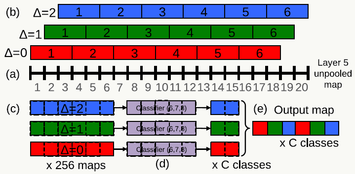
a图代表经过第5个卷积层后的feature map有20个神经元,选取stride=3做非重叠pooling,有以下3种方式:(通常我们只使用第一种)
> △=0分组:[1,2,3],[4,5,6],[7,8,9],...,[16,17,18]
> △=1分组:[2,3,4],[5,6,7],[8,9,10],...,[17,18,19]
> △=2分组:[3,4,5],[6,7,8],[9,10,11],...,[18,19,20]
在二维情况下,输入图像在经过FCN及第5个卷积层后得到若干个feature map,使用3x3 filter在feature map上做滑动窗口(注意此时不在原图上做,节省大量计算消耗)。按上图的原理,滑动窗口总共要做9次,从(0,0), (0,1), (0,2), (1,0), (1,1), (1,2), (2,0), (2,1), (2,2)处分别滑动。得到的feature map分别经过后面的3个FC层,得到多组特征,最后拼接起来得到最终特征向量并用于分类。
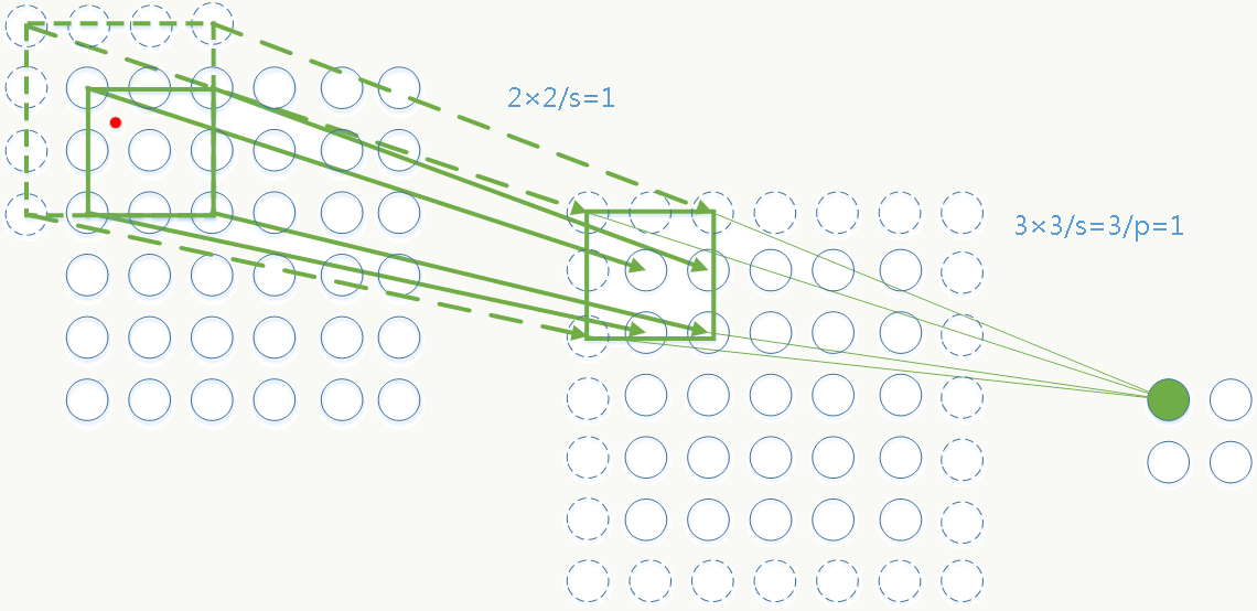
- Inference自适应输入图片大小
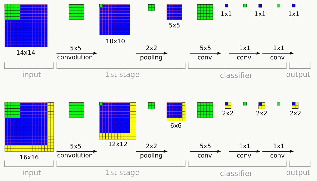
绿色代表卷积核,蓝色代表feature map,当输入大于规定尺寸时,在黄色区域会有额外计算,最终的输出也不是一个值而是一个矩阵,可以用各种策略输出最终结果,比如一种简单做法是用矩阵平均值作为最终分类结果。
8.2.2 OverFeat定位任务
回归训练
相对于分类问题,定位问题可以与其共享前1~5层网络结构,这种方式也被后面的模型所借鉴,区别是增加了一个\(l_2\)的回归损失函数,基本思路是对同一张图缩放产生多尺度图片做输入,用回归网络预测Bounding Box(后面简写为BB)后再做融合,需要注意回归层是与类别相关的,如果有1000个类则有1000个版本,每类一个。回归示意图如下:
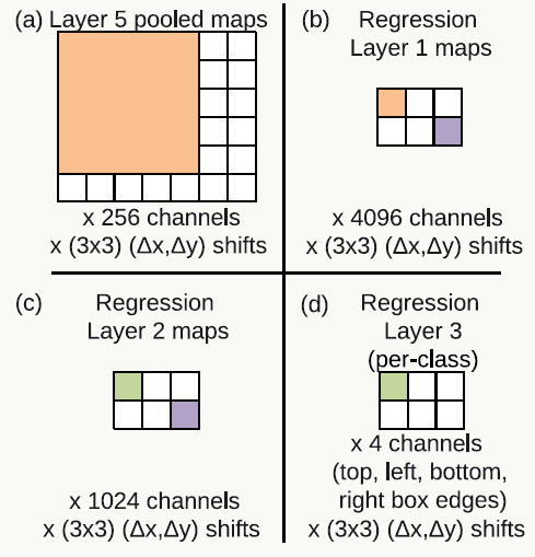
![]()
第5层pooling结果作为输入,共256个通道,以FCN的思想理解,先走一个4096通道的全连接层再走一个1024通道的全连接层,与前面类似使用Offet Pooing和滑动窗口对每类生成一个4通道矩阵,4个通道分别代表BB的四条边的坐标。
网络输出
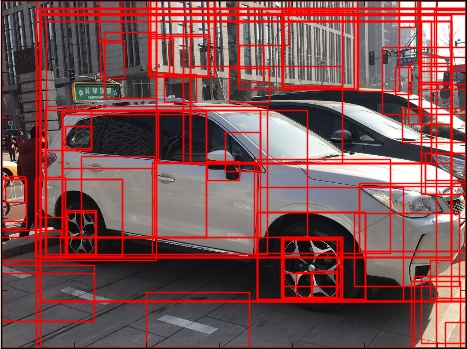
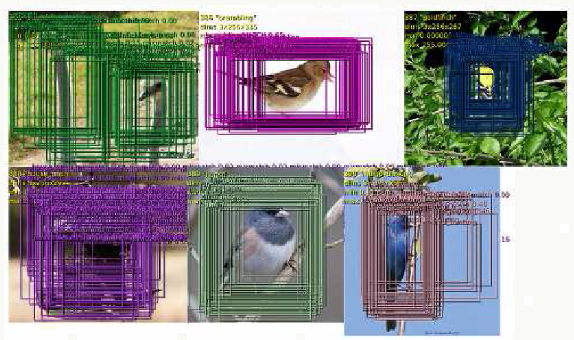
回归网络的输出例子如下,单图下生成多个BB的预测,这些BB倾向于收敛到一个固定位置并且可以定位物体姿势多样化的情况,当然计算复杂度不小,所以没法用到实时检测中。
![]()
预测融合策略
- 同一幅图在6种不同缩放尺度下分别输入分类网络,每种尺度下选top k类别作为标定,用\(C_s\)表示;
- 对任意尺度\(s\)分别输入BB 回归网络,用\(B_s\)表示每个类别对应的BB集合;
- 将所有\(B_s\)合并为大集合\(B\);
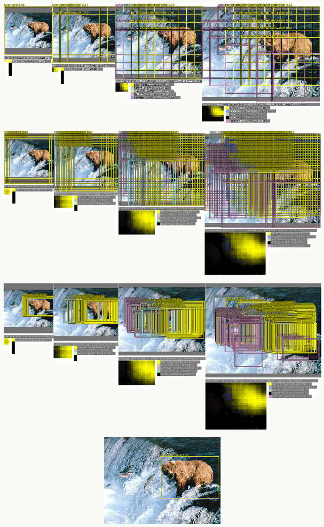
- 重复以下过程直到结束: \[ \begin{array}{l} (b_1^*,b_2^*)=argmin_{b_1\neq b_2 \in B}\text{match_score}(b_1,b_2)\\ if \quad \text{match_score}(b_1^*,b_2^*)>t \quad \\ then \quad stop.\\ Otherwise \quad set \quad B=B-\{b_1^*,b_2^*\}\cup \text{box_merge}(b_1^*,b_2^*) \end{array} \] 其中match_score为两个BB的中心点之间的距离及BB重合区域面积之和,box_merge为两个BB坐标均值,过程很好理解:所有分类(如可能有熊、鲸鱼等)的BB被放在一个大集合,多尺度得到的分类集合中,正确分类会占有优势(置信度、匹配度、BB连续度等),随着迭代的过程正确分类的BB被加强,错误分类的BB被减弱直到消失,不过这个方法确实复杂,可以看到在后来的算法有各种改进和替换。
![]()
8.2.3 OverFeat检测任务
与分类类似但需要考虑位置信息,同样采用网络结构共享特征提取,在预测分类中还需要加“背景”这一类。
8.2.4 代码实践
可参见:OverFeat
8.3 R-CNN
过去若干年,目标检测使用的都是滑动窗口的方式,这种方式计算效率较差,另外以往CNN在ImageNet比赛分类问题的表现更加突出,如何利用这些成果以及ImageNet的大量训练数据去借力打力也是一个值得研究的课题。R-CNN由Ross Girshick等人在《Rich feature hierarchies for accurate object detection and semantic segmentation》中提出,OverFeat从某种程度可以看做R-CNN的特例,R-CNN在图像检测领域有很大的影响力,该算法的亮点在于:使用Selective Search代替传统滑动窗口方式生成候选框并使用CNN提取特征;把分类和回归方法同时应用在检测中;当训练数据不足时,通过预训练利用领域数据(知识)做transfer learning,在对象数据集上再应用fine-tuning继续训练。
8.3.1 IoU
IoU(intersection over union),是用来衡量Bounding Box定位精度的指标,它的定义类似Jaccard距离,假设A为人工标定的BB,B为预测的BB则: \[IOU=\frac{area(A \cap B)}{area(A \cup B)}\]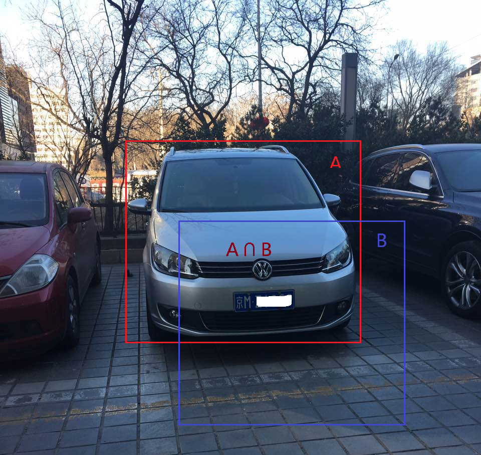
8.3.2 NMS
NMS(non-maximum suppression)在目标检测中用来依据置信度消除重叠度过高的重复候选框,从而提高检测算法效率。 例如,原图为: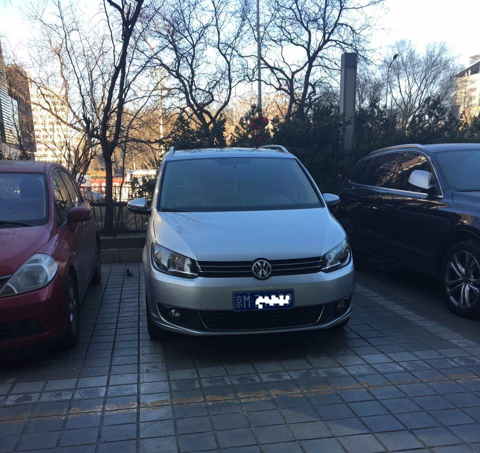
代码可参考:Non-Maximum Suppression for Object Detection in Python nms.py
1 | # import the necessary packages |
1 | # import the necessary packages |
8.3.3 mAP
先介绍什么是AP,以PASCAL VOC CHALLENGE 2010以后的定义做说明。 假设\(m\)个样本中有\(p\)个正例,依据包含正例的个数,可以得到\(p\)个recall值,分别为:\(1/p,2/p,3/p,...,p/p\),对于每个recall值\(r\)可以计算出对应\(r^{'} \geq r\)的最大precision,然后对这\(p\)个precision值取平均即得到AP值。 举个例子,假设是否为车的分类,一共有30个测试样本,预测结果及标注如下:
| 编号 | 预测值 | 实际值 |
|---|---|---|
| 1 | 0.88 | 1 |
| 2 | 0.76 | 0 |
| 3 | 0.56 | 0 |
| 4 | 0.92 | 0 |
| 5 | 0.10 | 1 |
| 6 | 0.77 | 1 |
| 7 | 0.23 | 0 |
| 8 | 0.34 | 0 |
| 9 | 0.35 | 0 |
| 10 | 0.66 | 1 |
| 11 | 0.56 | 0 |
| 12 | 0.45 | 1 |
| 13 | 0.93 | 1 |
| 14 | 0.97 | 0 |
| 15 | 0.81 | 1 |
| 16 | 0.78 | 0 |
| 17 | 0.66 | 0 |
| 18 | 0.54 | 0 |
| 19 | 0.43 | 1 |
| 20 | 0.31 | 0 |
| 21 | 0.22 | 0 |
| 22 | 0.12 | 0 |
| 23 | 0.02 | 0 |
| 24 | 0.05 | 1 |
| 25 | 0.15 | 0 |
| 26 | 0.01 | 0 |
| 27 | 0.77 | 1 |
| 28 | 0.37 | 0 |
| 29 | 0.43 | 1 |
| 30 | 0.99 | 1 |
按照预测得分降序排列后如下:
| 编号 | 预测值 | 实际值 |
|---|---|---|
| 30 | 0.99 | 1 |
| 14 | 0.97 | 0 |
| 13 | 0.93 | 1 |
| 4 | 0.92 | 0 |
| 1 | 0.88 | 1 |
| 15 | 0.81 | 1 |
| 16 | 0.78 | 0 |
| 6 | 0.77 | 1 |
| 27 | 0.77 | 1 |
| 2 | 0.76 | 0 |
| 10 | 0.66 | 1 |
| 17 | 0.66 | 0 |
| 3 | 0.56 | 0 |
| 11 | 0.56 | 0 |
| 18 | 0.54 | 0 |
| 12 | 0.45 | 1 |
| 19 | 0.43 | 1 |
| 29 | 0.43 | 1 |
| 28 | 0.37 | 0 |
| 9 | 0.35 | 0 |
| 8 | 0.34 | 0 |
| 20 | 0.31 | 0 |
| 7 | 0.23 | 0 |
| 21 | 0.22 | 0 |
| 25 | 0.15 | 0 |
| 22 | 0.12 | 0 |
| 5 | 0.10 | 1 |
| 24 | 0.05 | 1 |
| 23 | 0.02 | 0 |
| 26 | 0.01 | 0 |
| 编号 | 预测值 | 实际值 | Precision | Recall(r) | Max Precision with Recall(r'≥r) | AP |
| 30 | 0.99 | 1 | 1/1=1 | 1/12=0.08 | 1 | 0.609 |
| 14 | 0.97 | 0 | 1/2=0.5 | 1/12=0.08 | ||
| 13 | 0.93 | 1 | 2/3=0.67 | 2/12=0.17 | 0.67 | |
| 4 | 0.92 | 0 | 2/4=0.5 | 2/12=0.17 | ||
| 1 | 0.88 | 1 | 3/5=0.6 | 3/12=0.25 | 0.6 | |
| 15 | 0.81 | 1 | 4/6=0.67 | 4/12=0.33 | 0.67 | |
| 16 | 0.78 | 0 | 4/7=0.57 | 4/12=0.33 | ||
| 6 | 0.77 | 1 | 5/8=0.63 | 5/12=0.42 | 0.63 | |
| 27 | 0.77 | 1 | 6/9=0.67 | 6/12=0.5 | 0.67 | |
| 2 | 0.76 | 0 | 6/10=0.6 | 6/12=0.5 | ||
| 10 | 0.66 | 1 | 7/11=0.64 | 7/12=0.58 | 0.64 | |
| 17 | 0.66 | 0 | 7/12=0.58 | 7/12=0.58 | ||
| 3 | 0.56 | 0 | 7/13=0.54 | 7/12=0.58 | ||
| 11 | 0.56 | 0 | 7/14=0.5 | 7/12=0.58 | ||
| 18 | 0.54 | 0 | 7/15=0.47 | 7/12=0.58 | ||
| 12 | 0.45 | 1 | 8/16=0.5 | 8/12=0.67 | 0.5 | |
| 19 | 0.43 | 1 | 9/17=0.53 | 9/12=0.75 | 0.53 | |
| 29 | 0.43 | 1 | 10/18=0.56 | 10/12=0.83 | 0.56 | |
| 28 | 0.37 | 0 | 10/19=0.53 | 10/12=0.83 | ||
| 9 | 0.35 | 0 | 10/20=0.5 | 10/12=0.83 | ||
| 8 | 0.34 | 0 | 10/21=0.48 | 10/12=0.83 | ||
| 20 | 0.31 | 0 | 10/22=0.45 | 10/12=0.83 | ||
| 7 | 0.23 | 0 | 10/23=0.43 | 10/12=0.83 | ||
| 21 | 0.22 | 0 | 10/24=0.42 | 10/12=0.83 | ||
| 25 | 0.15 | 0 | 10/25=0.4 | 10/12=0.83 | ||
| 22 | 0.12 | 0 | 10/26=0.38 | 10/12=0.83 | ||
| 5 | 0.1 | 1 | 11/27=0.41 | 11/12=0.92 | 0.41 | |
| 24 | 0.05 | 1 | 12/28=0.43 | 12/12=1 | 0.43 | |
| 23 | 0.02 | 0 | 12/29=0.41 | 12/12=1 | ||
| 26 | 0.01 | 0 | 12/30=0.4 | 12/12=1 |
mAP是所有类别下的AP求算数平均值的结果。
8.3.4 R-CNN原理
训练阶段 整个过程分4步: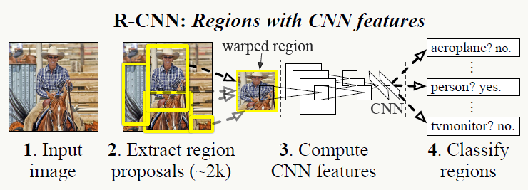
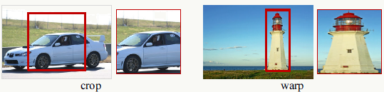
- 候选框生成阶段 利用Selective Search生成2000个候选框(BB),之前很多年人们用的都是滑动窗口方式。需要注意的是,由于候选框图片大小不一,而后续用于提特征的CNN对输入要求是固定大小的(227×227),所以需要做预处理,文中实验效果最好的方法是:不论长宽比例直接将图片缩放到227×227大小,并做padding=16的处理以保留上下文信息。
- 特征提取阶段 利用CNN提取图片特征,文中大部分实验结果采用AlexNet网络结构,小部分采用VGG16,前者训练速度快但精度相对低,后者反之,AlexNet结构如下。
![]()
- 有监督预训练 使用ImageNet ILSVRC2012分类任务的1000类训练数据训练一个AlexNet模型,由于CNN主要作用体现在特征提取中,同样是猫狗,在不同数据集上特征是一样的,所以可以在不同问题间共享特征,区别无非在最终任务目标和特征如何组合上;
- 基于领域知识的fine-tuning 以上述模型做权重初始化,将softmax层1000类输出改为随机初始化权重的N+1类输出(1为背景类,对VOC,N=20),在目标训练集上继续训练,其中正样本为:与ground truth框IoU≥0.5的样本,其余的为负样本。训练时优化器采用学习率为0.001的SGD,样本采用mini-batch方式学习,大小为128,其中每个batch由采用均匀分布随机抽取的针对所有分类的32个正样本和96个负样本(背景)组成。
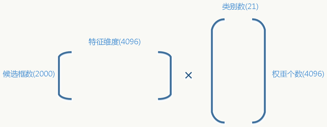
- 训练分类器阶段 每一类做一个线性SVM分类器(为配合候选框特征向量的维度,每个SVM分类器为4096个权重),正样本为:每一类的ground truth,负样本为:与ground truth的IoU≤0.3的候选框(0.3这个阈值是通过在{0,0.1,0.2,0.3,0.4,0.5}集合上做grid search后观察验证集效果得到的)。 例如,对于VOC:
![]()
- 训练回归器阶段 主要目的是修正BB减少定位错误,借鉴DPM的方法,使用ridge regression修正BB位置,具体方法为: 假设输入为:候选框与ground truth框对集合,用\(\{(P^i,G^i)\}_{i=1,...,N}\),其中\(P_i=(P_x^i,P_y^i,P_w^i,P_h^i)\),括号中分别为候选框中心点的坐标及候选框宽与高,选取靠近(IoU≥0.6)ground truth的候选框,目标是学习一个映射使得候选框能被修正到ground truth框。利用SIT(scale-invariant translation)和LST(log-space translation)思想去学习这个变换(这里大家可以想想为什么?): \[ \begin{array}{l} \hat{G_x}=P_w\cdot d_x(P)+P_x\\ \hat{G_y}=P_h\cdot d_y(P)+P_y \\ \hat{G_w}=P_w\cdot e^{d_w(P)}\\ \hat{G_h}=P_h\cdot e^{d_h(P)} \end{array} \] 变换函数\(d_*(P)\)与AlexNet最后一个pooling层(4096个特征)的输出\(\phi_5(P)\)关系为: \[d_*(P)=w^T_*\phi_5(P)\] 优化目标函数为: \[w_*=argmin_{\hat{w_*}}\sum_i^N(t_*^i-\hat{w}_*^T\phi_5(P^i))^2+\lambda||\hat{w_*}||^2\] 其中: \[ \begin{array}{l} t_x=(G_x-P_x)/P_w\\ t_y=(G_y-P_y)/P_h \\ t_w=log(G_w/P_w)\\ t_h=log(G_h/P_h) \end{array} \]
以上四个步骤是相互独立的,后验(马后炮)的来看,可以做这些改进:
1、把分类和回归放在一个网络做共享特征;
2、网络结构对输入图片大小自适应;
3、把候选框生成算法也放在同一个网络来做共享特征;
4、分类器抛弃SVM直接融合在神经网络中;
5、不用每个候选框都做一次特征提取。
测试阶段过程如下:
- 使用SS提取2000个候选框
- 将候选框大小缩放到227×227
- 每个候选框输入CNN,产生特征后对每一类做SVM分类输出置信度
- 对候选框做基于贪心的NMS
- 每个候选框的BB只做一次预测
8.3.5 代码实践
作者代码能力极强,具体可见:R-CNN: Region-based Convolutional Neural Networks。
8.4 SPP-Net
SPP-Net是何凯明等人在《Spatial Pyramid Pooling in Deep Convolutional Networks for Visual Recognition》一文中提出,文章亮点是主要解决了两个问题:
1、允许CNN网络的输入图片大小不固定(后面的FCN也可以解决这个问题);
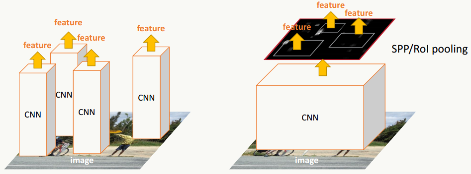
2、借鉴OverFeat只对整张图做一次特征提取,一些操作只在feature map上做而不用在原图进行且feature map上的点可以还原到原图上。
8.4.1 问题回顾
之前的CNN网络的输入都是固定大小的,好处是网络结构相对简单和计算量低,坏处是所有图片都需要做预处理,这个会损失原图信息或引入噪声。训练和预测的一般流程是:

8.4.2 SPP详解
可以把这个问题看做如何找到输入可变,输出固定且能保留空间信息的映射问题,问题三个相关变量:feature map的大小、bin的个数(借鉴BoW《Video Google: A Text Retrieval Approach to Object Matching in Videos》的思想,表示固定特征的维度数)、pooling步长。现在feature map的大小不固定但bin的个数固定,于是唯一能自适应可变的就是pooling步长了。 假设:最后一个卷积层产生的feature map大小为\(a×a\),希望产生\(n×n\)个bins,则窗口大小为\(\lceil\frac{a}{n}\rceil\),步长为\(\lfloor\frac{a}{n}\rfloor\),例如: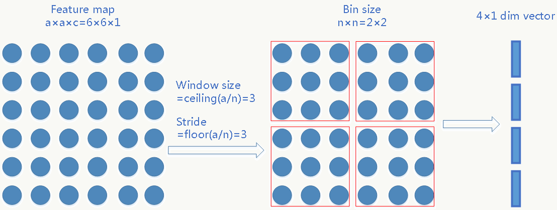
每个bin的pooling方式可以是max pooling或其他pooling。
SPP同样支持多尺度特征,例如4×4、2×2、1×1三种尺度最后拼成21×256维特征向量: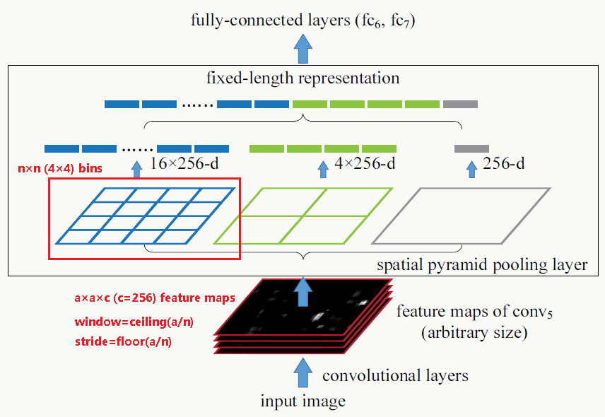
8.4.3 感受野(Receptive Field)
感受野来源于生物学,Levine and Shefner在《Fundamentals of sensation and perception》中将感受野定义为:由于受到刺激导致特定神经元发生反应的区域。比如人在观察某个物体的某个部分时由于受到刺激,物体会投影到视网膜,之后传到给大脑并激活某个区域(橘色的框框住的区域)。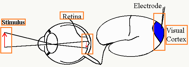
感受野的大小与以下两个因素有关但与是否padding无关: 1、filter的大小; 2、stride的大小。
8.4.4 feature map与原图对应关系转换
由于SPP只对原图做一次特征提取,省去了大量重复劳动,另外由于特征点的可还原性,使得后续对所有对候选框做SPP特征映射操作时只需要在最后一个卷积层产生的feature map上进行即可(否则需要考虑感受野上的所有特征映射将会产生巨大的计算量)。 详情可参考《R-CNN minus R》. 简单的转换方法为: 需要对CNN网络的所有卷积层和pooling层做padding,使得原图中的任何一点与卷积或pooling后的图上的点一一对应(边缘信息也没有丢失)。
假设:
1、任何一层的核大小为\(p\);
2、每层padding值为\(\lfloor\frac{p}{2}\rfloor\);
3、原图中任何一点坐标为\((x,y)\),该点在任何一个feature map上的位置为\((x,^{'},y^{'})\);
4、从原图到该feature map感受野范围内的所有stride乘积为\(S\)。
则: 原图候选框左上点的坐标与其在任意feature map上的坐标关系为: \[ \begin{array}{l} x^{'}=\lfloor\frac{x}{S}\rfloor+1\\ y^{'}=\lfloor\frac{y}{S}\rfloor+1 \end{array} \] 原图候选框右下点的坐标与其在任意feature map上的坐标关系为: \[ \begin{array}{l} x^{'}=\lceil\frac{x}{S}\rceil-1\\ y^{'}=\lceil\frac{y}{S}\rceil-1 \end{array} \]
通用的转换方法为: \[ \begin{array}{l} i_0=\alpha_L(i_L-1)+\beta_L\\ \alpha_L=\prod_{p=1}^L S_p\\ \beta_L=1+\sum_{p=1}^L(\prod_{q=1}^{p-1}S_q)(\frac{F_p-1}{2}-P_p) \end{array} \] 其中: \(i_0\)是feature map上的特征点\(i_L\)在感受野的中心位置坐标; \(L\)是当前特征点处于由CNN的第几层产生的feature map中; \(S_p\)第\(p\)层的stride大小; \(F_p\)第\(p\)层的filter大小; \(P_p\)第\(p\)层的padding大小。 反过来可以知道原图任何一个候选框在任何一个feature map上的位置。
感受野大小的计算采用Top to Down的方式,从当前层往靠近输入层的方式逐层传递,具体方法为: 假设:待计算感受野的特征点所在feature map所处层为\(L\),\(r_0\)为特征点在原图的感受野大小。 则: \[ \begin{array}{l} r_L=1;\\ for \quad t=L;t<=1;t--\\ \quad \quad \quad r_{t-1}=(r_{t}-1)*S_{t}+F_{t};\\ return \quad r_0; \end{array} \]
以下面两幅图为例:
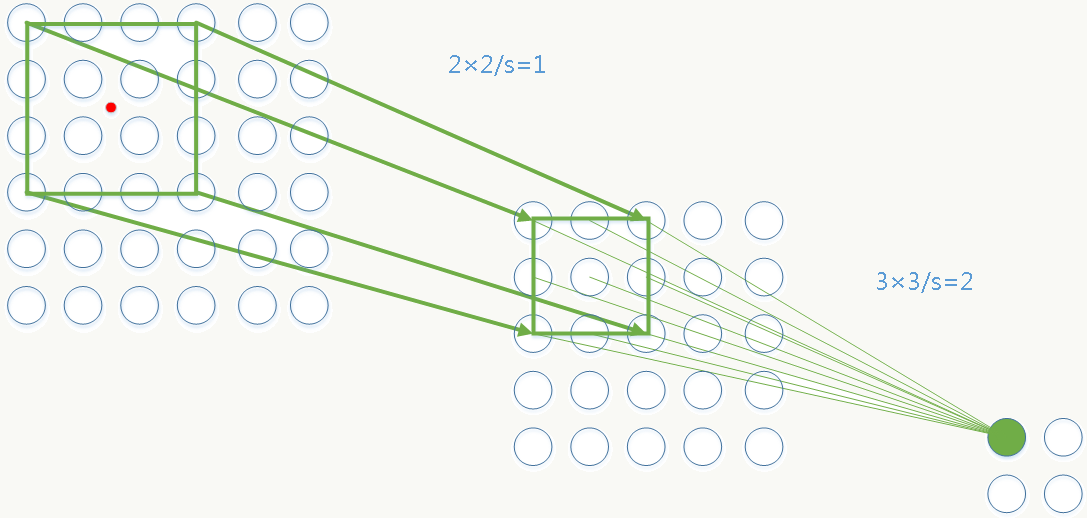
图一 无padding。
![]()
绿色点为第2层feature map上坐标为(1,1)的点,则它在原图的中心点为: \[ \begin{array}{l} \alpha_2=1*2=2\\ \beta_2=1+(2-1)/2+1*(3-1)/2=2.5\\ i_0=2*(i_2-1)+2.5 \end{array} \] 中心点坐标为图中红点:(2.5,2.5) 感受野大小为4: \[ \begin{array}{l} r_2=1\\ r_1=(r_2-1)*2+3=3\\ r_0=(r_1-1)*1+2=4 \end{array} \]
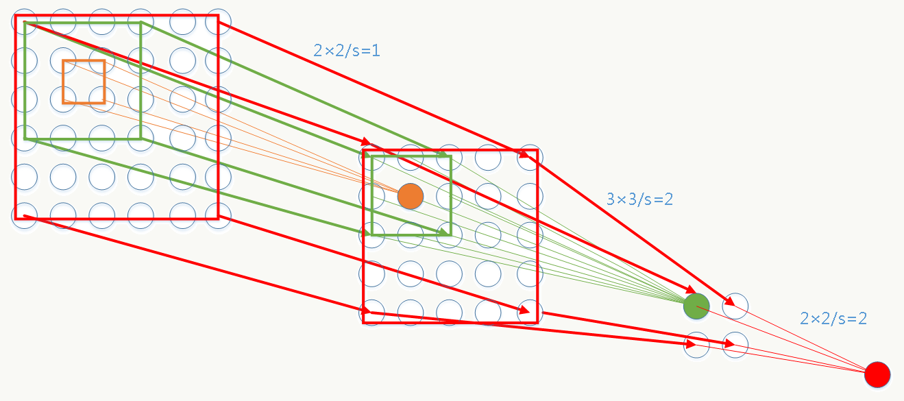
图二 第一层有padding。
![]()
绿色点为第2层feature map上坐标为(1,1)的点,则它在原图的中心点为: \[ \begin{array}{l} \alpha_2=1*3=3\\ \beta_2=1+(2-1)/2+1*((3-1)/2-1)=1.5\\ i_0=3*(i_2-1)+1.5 \end{array} \] 中心点坐标为图中红点:(1.5,1.5) 感受野大小为4: \[ \begin{array}{l} r_2=1\\ r_1=(r_2-1)*3+3=3\\ r_0=(r_1-1)*1+2=4 \end{array} \]
8.4.5 代码实践
- receptivefield.py
1
2
3
4
5
6
7
8
9
10
11
12
13
14
15
16
17
18
19
20
21
22
23
24
25
26
27
28
29
30
31
32
33
34
35
36
37
38
39
40
41
42
43
44
45
46
47
48
49
50
51
52
53
54
55
56
57
58
59
60
61
62
63
64
65
66
67
68
69
70
71
72
73
74
75
76
77
78
79
80
81
82
83
84
85
86
87
88
89# -*- coding: utf-8 -*-
#一层表示为一个三元组: [filter size, stride, padding]
import math
def forword(conv, layerIn):
n_in = layerIn
k = conv[0]
s = conv[1]
p = conv[2]
return math.floor((n_in - k + 2*p)/s) + 1
def alexnet():
convnet = [[],[11,4,0],[3,2,0],[5,1,2],[3,2,0],[3,1,1],[3,1,1],[3,1,1],[3,2,0],[6,1,0], [1, 1, 0]]
layer_names = [['input'],'conv1','pool1','conv2','pool2','conv3','conv4','conv5','pool5','fc6-conv', 'fc7-conv']
return [convnet, layer_names]
def testnet():
convnet = [[],[2,1,0],[3,3,1]]
layer_names = [['input'],'conv1','conv2']
return [convnet, layer_names]
# layerid >= 1
def receptivefield(net, layerid):
if layerid > len(net[0]):
print '[error] receptivefield:no such layerid!'
return 0
rf = 1
for i in reversed(range(layerid)):
filtersize, stride, padding = net[0][i+1]
rf = (rf - 1)*stride + filtersize
print ' 感受野大小为:%d.' % (int(rf))
return rf
def anylayerout(net, layerin, layerid):
if layerid > len(net[0]):
print '[error] anylayerout:no such layerid!'
return 0
for i in range(layerid):
if i == 0:
fout = forword(net[0][i+1], layerin)
continue
fout = forword(net[0][i+1], fout)
print '当前层为:%s, 输出节点维度为:%d.' % (net[1][layerid], int(fout))
#x,y>=1
def receptivefieldcenter(net, layerid, x, y):
if layerid > len(net[0]):
print '[error] receptivefieldcenter:no such layerid!'
return 0
al = 1
bl = 1
for i in range(layerid):
filtersize, stride, padding = net[0][i+1]
al = al * stride
ss = 1
for j in range(i):
fsize, std, pad = net[0][j+1]
ss = ss * std
bl = bl + ss * (float(filtersize-1)/2 - padding)
xi0 = al * (x - 1) + float(bl)
yi0 = al * (y - 1) + bl
print ' 该层上的特征点(%d,%d)在原图的感受野中心坐标为:(%.1f,%.1f).' % (int(x), int(y), float(xi0), float(yi0))
return (xi0, yi0)
# net:为某个CNN网络
# insize:为输入层大小
# totallayers:为除了输入层外的所有层个数
# x,y为某层特征点坐标
def printlayer(net, insize, totallayers, x, y):
for i in range(totallayers):
# 计算每一层的输出大小
anylayerout(net, insize, i+1)
# 计算每层的感受野大小
receptivefield(net, i+1)
# 计算feature map上(x,y)点在原图感受野的中心位置坐标
receptivefieldcenter(net, i+1, x, y)
if __name__ == '__main__':
#net = testnet()
#printlayer(net, insize=6, totallayers=2, x=1, y=1)
net = alexnet()
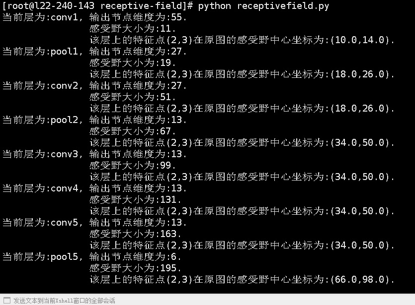
printlayer(net, insize=227, totallayers=8, x=2, y=3) - 输出
![]()
8.5 Fast R-CNN
《Fast R-CNN》的出现解决了R-CNN+SPP中的以下问题:
- 把分类和回归放在一个网络做共享特征,提取的特征向量不用落地
- 借鉴SPP,网络结构对输入图片大小自适应
- 抛弃SVM分类器,利用softmax直接融合在神经网络中
- 借鉴SPP,只做一次全图的特征提取,不用每个候选框都做
8.5.1 算法概述
算法基本步骤为: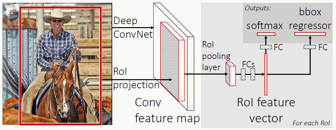
- 候选框生成阶段 方法同R-CNN。
- 特征提取阶段 注意整个网络的输入为两部分:整个图和候选框信息。特征提取会对整张图进行,利用输入的候选框坐标及大小信息可以方便低成本的在任何一个feature map上找到任何一个原图点的特征映射点(方法回看SPP-net),大大提高了特征提取效率。
- RoI pooling阶段 借鉴SPP的思想,对每个候选框生成一个自适应候选框大小的固定长度的ROI(region of interest)特征向量,除此之外,大家还可以想想RoI Pooling的更深层次作用。
- 多任务学习阶段 把得到的RoI特征向量用全连接层做组合后分别送入两个分支:一个做分类,一个做Bounding Box回归,并为此设计一个多任务损失函数。
8.5.2 训练阶段
RoI pooling层生成说明
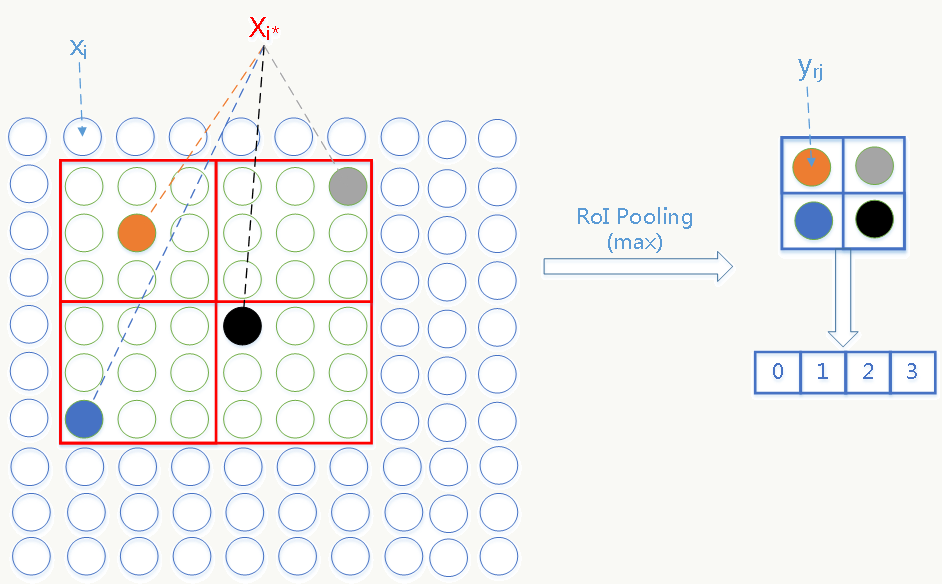
RoI pooling是SPP的特殊形式(金字塔层数为1,pooling采用max pooling),具体原理类比SPP即可,feature map通过该层后会产生\(H × W\)大小(例如7 × 7)的特征向量,例如: 某个RoI坐标表示为四元组\((r,c,h,w)\),其中\(r,c\)为RoI最左上角坐标,\(h,w\)为其高与宽,则RoI pooling会划分\(H × W\)个大小\(为\frac{h}{H} × \frac{w}{W}\)的小网格,之后对每个小网格做max pooling即可。
RoI pooling层反向传播
RoI pooling的反向传播比较简单,输入feature map上的任意特征元素的梯度信息为:所有由它产生的roi pooling feature map的特征元素所带梯度信息的累加和。
![]()
假设:
1、\(x_i \in R\)是 RoI pooling层输入feature map的第\(i\)个特征元素;
2、\(y_{rj}\)是第\(r\)个RoI的roi pooling后得到feature map的第\(j\)个特征元素;
3、\(R(r,j)\)是第\(r\)个RoI通过roi pooling得到的feature map上的第\(j\)个输出特征元素对应原feature map上的子图;
\(i^*_{r,j}=argmax_{i^{\text{'}} \in R(r,j)}x_i^\text{'}\)为在上述子图中做max pooling后得到的原feature map元素索引号。
则反向传播得到的原feature map元素的梯度为: \[ \frac{\partial L}{\partial x_i}=\sum_r \sum_j[i=i^*_{r,j}]\frac{\partial L}{\partial y_{rj}} \] \([x]\)函数表示:如果\(x\)为真则返回1,否则返回0。
多任务损失函数
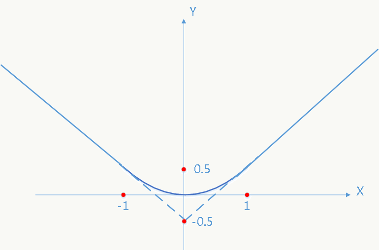
使用smooth L1函数并融合分类和bounding box回归损失,损失函数如下: \[ L(p,u,t^u,v)=L_{cls}(p,u)+\lambda \cdot [u \geq 1]L_{loc}(t^u,v) \] 其中: \[L_{cls}(p,u)=-log \text{ }p_u\] \[L_{loc}(t^u,v)=\sum_{i \in \{x,y,w,h\}}smooth_{L_1}(t_i^u-v_i)\]
\[ smooth_{L_1}(x)= \begin{cases} 0.5x^2& \text{if |x|<1}\\ |x|-0.5& \text{otherwise} \end{cases} \] smooth L1函数对异常点不敏感(在|x|值较大时使用线性分段函数而不是二次函数),如图:
![]()
8.5.3 代码实践
fast r-cnn完整代码请参考rbgirshick/fast-rcnn。
- RoI Pooling层实现解析
1
2
3
4
5
6
7
8
9
10
11
12
13
14
15
16
17
18
19
20
21
22
23
24
25
26
27
28
29
30
31
32
33
34
35
36
37
38
39
40
41
42
43
44
45
46
47
48
49
50
51
52
53
54
55
56
57
58
59
60
61
62
63
64
65
66
67
68
69
70
71
72
73
74
75
76
77
78
79
80
81
82
83
84
85
86
87
88
89
90
91
92
93
94
95
96
97
98
99
100
101
102
103
104
105
106
107
108
109
110
111
112
113
114
115
116
117
118
119
120
121
122
123
124
125
126
127
128
129
130
131
132
133
134
135
136
137
138
139
140
141
142
143
144
145
146
147
148
149
150
151
152
153
154
155
156
157
158
159
160
161
162
163
164
165
166
167
168
169
170
171
172
173
174
175
176
177
178
179
180
181
182
183
184
185
186
187
188
189
190
191
192
193
194
195
196
197
198
199
200
201
202
203
204
205
206
207
208
209
210
211
212
213
214
215
216
217
218
219
220
221
222
223
224
225
226
227
228
229
230
231
232
233
234
235
236
237
238
239
240
241
242
243
244
245
246
247
248
249
250
251
252
253
254
255
256
257
258
259
260
261
262
263
264
265
266
267
268// ------------------------------------------------------------------
// Fast R-CNN
// Copyright (c) 2015 Microsoft
// Licensed under The MIT License [see fast-rcnn/LICENSE for details]
// Written by Ross Girshick
// ------------------------------------------------------------------
using std::max;
using std::min;
namespace caffe {
template <typename Dtype>
// 以下参数解释以VGG16为例,即进入roi pooling前的网络结构采用经典VGG16.
// 在Layer类中输入数据用bottom表示, 输出数据用top表示
__global__ void ROIPoolForward(
const int nthreads, // 任务数,对应通过roi pooling后的输出feature map的神经元节点总数,
// 具体为:RoI的个数(m) × channel个数(VGG16的conv5_3的输出为512个) × roi pooling输出宽(配置为7) × roi pooling输出高(配置为7) = 25088×m个
const Dtype* bottom_data, // 输入的feature map,原图经过各种卷积、pooling等前向传播后得到(VGG16的conv5_3卷积产生的feature map,大小为:512×14×14)
const Dtype spatial_scale, // 由之前所有卷积层的strides相乘得到,在fast rcnn中为1/16,注:从原图往conv5_3的feature map上映射为缩小过程,所以乘以1/16,反之需要乘以16
const int channels, // 输入层(VGG16为卷积层conv5_3)feature map的channel个数(512)
const int height, // 输入层(VGG16为卷积层conv5_3)feature map的高(14)
const int width, // 输入层(VGG16为卷积层conv5_3)feature map的宽(14)
const int pooled_height, // roi pooling输出feature map的高,fast rcnn中配置为h=7
const int pooled_width, // roi pooling输出feature map的宽,fast rcnn中配置为w=7
const Dtype* bottom_rois, // 输入的roi信息,存储所有rois或一个batch的rois,数据结构为[batch_ind,x1,y1,x2,y2],包含roi的:索引、左上角坐标及右下角坐标
Dtype* top_data, // 存储roi pooling后得到的feature map
int* argmax_data) { // 为每个roi pooling后的feature map元素存储max pooling后对应conv5_3 feature map元素的索引信息,长度等于nthreads
// index为线程索引,个数为roi pooling后的feature map上所有值的个数,索引范围为:[0,nthreads-1]
CUDA_KERNEL_LOOP(index, nthreads) {
// 该线程对应的top blob(N,C,H,W)中的W,输出roi pooling后feature map的中的宽的坐标,即feature map的第i=[0,k-1]列
int pw = index % pooled_width;
// 该线程对应的top blob(N,C,H,W)中的H,输出roi pooling后feature map的中的高的坐标,即feature map的第j=[0,k-1]行
int ph = (index / pooled_width) % pooled_height;
// 该线程对应的top blob(N,C,H,W)中的C,即第c个channel,channel数最大值为输入feature map的channel数(VGG16中为512).
int c = (index / pooled_width / pooled_height) % channels;
// 该线程对应的是第几个RoI,一共m个.
int n = index / pooled_width / pooled_height / channels;
// [start, end),指定RoI信息的存储范围,指针每次移动5的倍数是因为包含信息的数据结构大小为5,包含信息为:[batch_ind,x1,y1,x2,y2],含义同上
bottom_rois += n * 5;
// 将每个原图的RoI区域映射到feature map(VGG16为conv5_3产生的feature mao)上的坐标,bottom_rois第0个位置存放的是roi索引.
int roi_batch_ind = bottom_rois[0];
// 原图到feature map的映射为乘以1/16,这里采用粗映射而不是上文讲的精确映射,原因你懂的.
int roi_start_w = round(bottom_rois[1] * spatial_scale);
int roi_start_h = round(bottom_rois[2] * spatial_scale);
int roi_end_w = round(bottom_rois[3] * spatial_scale);
int roi_end_h = round(bottom_rois[4] * spatial_scale);
// 强制把RoI的宽和高限制在1x1,防止出现映射后的RoI大小为0的情况
int roi_width = max(roi_end_w - roi_start_w + 1, 1);
int roi_height = max(roi_end_h - roi_start_h + 1, 1);
// 根据原图映射得到的roi的高和配置的roi pooling的高(这里大小配置为7)自适应计算bin桶的高度
Dtype bin_size_h = static_cast<Dtype>(roi_height)
/ static_cast<Dtype>(pooled_height);
// 根据原图映射得到的roi的宽和配置的roi pooling的宽(这里大小配置为7)自适应计算bin桶的宽度
Dtype bin_size_w = static_cast<Dtype>(roi_width)
/ static_cast<Dtype>(pooled_width);
// 计算第(i,j)个bin桶在feature map上的坐标范围,需要依据它们确定后续max pooling的范围
int hstart = static_cast<int>(floor(static_cast<Dtype>(ph)
* bin_size_h));
int wstart = static_cast<int>(floor(static_cast<Dtype>(pw)
* bin_size_w));
int hend = static_cast<int>(ceil(static_cast<Dtype>(ph + 1)
* bin_size_h));
int wend = static_cast<int>(ceil(static_cast<Dtype>(pw + 1)
* bin_size_w));
// 确定max pooling具体范围,注意由于RoI取自原图,其左上角不是从(0,0)开始,
// 所以需要加上 roi_start_h 或 roi_start_w作为偏移量,并且超出feature map尺寸范围的部分会被舍弃
hstart = min(max(hstart + roi_start_h, 0), height);
hend = min(max(hend + roi_start_h, 0), height);
wstart = min(max(wstart + roi_start_w, 0), width);
wend = min(max(wend + roi_start_w, 0), width);
bool is_empty = (hend <= hstart) || (wend <= wstart);
// 如果区域为0返回错误代码
Dtype maxval = is_empty ? 0 : -FLT_MAX;
// If nothing is pooled, argmax = -1 causes nothing to be backprop'd
int maxidx = -1;
bottom_data += (roi_batch_ind * channels + c) * height * width;
// 在给定bin桶的区域中做max pooling
for (int h = hstart; h < hend; ++h) {
for (int w = wstart; w < wend; ++w) {
int bottom_index = h * width + w;
if (bottom_data[bottom_index] > maxval) {
maxval = bottom_data[bottom_index];
maxidx = bottom_index;
}
}
}
// 为某个roi pooling的feature map元素记录其由对conv5_3(VGG16)的feature map做max pooling后产生元素的索引号及值
top_data[index] = maxval;
argmax_data[index] = maxidx;
}
}
template <typename Dtype>
void ROIPoolingLayer<Dtype>::Forward_gpu(
const vector<Blob<Dtype>*>& bottom, // 以VGG16为例,bottom[0]为最后一个卷积层conv5_3产生的feature map,shape[1, 512, 14, 14],
// bottom[1]为rois数据,shape[roi个数m, 5]
const vector<Blob<Dtype>*>& top) { // top为输出层结构, top->count() = top.n(RoI的个数) × top.channel(channel数)
// × top.w(输出feature map的宽) × top.h(输出feature map的高)
const Dtype* bottom_data = bottom[0]->gpu_data();
const Dtype* bottom_rois = bottom[1]->gpu_data();
Dtype* top_data = top[0]->mutable_gpu_data();
int* argmax_data = max_idx_.mutable_gpu_data();
int count = top[0]->count();
/*
参照caffe-fast-rcnn/src/caffe/layers/roi_pooling_layer.cpp中的代码:
template <typename Dtype>
void ROIPoolingLayer<Dtype>::Reshape(const vector<Blob<Dtype>*>& bottom,
const vector<Blob<Dtype>*>& top) {
channels_ = bottom[0]->channels();
height_ = bottom[0]->height();
width_ = bottom[0]->width();
top[0]->Reshape(bottom[1]->num(), channels_, pooled_height_, pooled_width_);
max_idx_.Reshape(bottom[1]->num(), channels_, pooled_height_, pooled_width_);
}*/
/*
参照caffe-fast-rcnn/include/caffe/util/device_alternate.hpp中的代码:
// CUDA_KERNEL_LOOP
#define CUDA_KERNEL_LOOP(i, n) \
for (int i = blockIdx.x * blockDim.x + threadIdx.x; \
i < (n); \
i += blockDim.x * gridDim.x)
// CAFFE_GET_BLOCKS
// CUDA: number of blocks for threads.
inline int CAFFE_GET_BLOCKS(const int N) {
return (N + CAFFE_CUDA_NUM_THREADS - 1) / CAFFE_CUDA_NUM_THREADS;
}
// CAFFE_CUDA_NUM_THREADS
// CUDA: thread number configuration.
// Use 1024 threads per block, which requires cuda sm_2x or above,
// or fall back to attempt compatibility (best of luck to you).
#if __CUDA_ARCH__ >= 200
const int CAFFE_CUDA_NUM_THREADS = 1024;
#else
const int CAFFE_CUDA_NUM_THREADS = 512;
#endif
*/
ROIPoolForward<Dtype><<<CAFFE_GET_BLOCKS(count), CAFFE_CUDA_NUM_THREADS>>>(
count, bottom_data, spatial_scale_, channels_, height_, width_,
pooled_height_, pooled_width_, bottom_rois, top_data, argmax_data);
CUDA_POST_KERNEL_CHECK;
}
template <typename Dtype>
// 反向传播的过程与论文中"Back-propagation through RoI pooling layers"这一小节的公式完全一致
__global__ void ROIPoolBackward(
const int nthreads, // 输入feature map的元素数(VGG16为:512×14×14)
const Dtype* top_diff, // roi pooling输出feature map所带的梯度信息∂L/∂y(r,j)
const int* argmax_data, // 同前向,不解释
const int num_rois, // 同前向,不解释
const Dtype spatial_scale, // 同前向,不解释
const int channels, // 同前向,不解释
const int height, // 同前向,不解释
const int width, // 同前向,不解释
const int pooled_height, // 同前向,不解释
const int pooled_width, // 同前向,不解释
Dtype* bottom_diff, // 保留输入feature map每个元素通过梯度反向传播得到的梯度信息
const Dtype* bottom_rois) { // 同前向,不解释
// 含义同前向,需要注意的是这里表示的是输入feature map的元素数(反向传播嘛)
CUDA_KERNEL_LOOP(index, nthreads) {
// 同前向,不解释
int w = index % width;
int h = (index / width) % height;
int c = (index / width / height) % channels;
int n = index / width / height / channels;
Dtype gradient = 0;
// 同论文中公式,任何一个输入feature map的元素的梯度信息为:
// 所有max pooling时被该元素落入且该元素值被选中(最大值)的
// roi pooling feature map元素的梯度信息累加和
// 遍历所有RoI,以判断是否满足上述条件
for (int roi_n = 0; roi_n < num_rois; ++roi_n) {
const Dtype* offset_bottom_rois = bottom_rois + roi_n * 5;
int roi_batch_ind = offset_bottom_rois[0];
// 如果RoI的索引号不满足条件则跳过
if (n != roi_batch_ind) {
continue;
}
// 找原图RoI在feature map上的映射位置,解释同前向传播
int roi_start_w = round(offset_bottom_rois[1] * spatial_scale);
int roi_start_h = round(offset_bottom_rois[2] * spatial_scale);
int roi_end_w = round(offset_bottom_rois[3] * spatial_scale);
int roi_end_h = round(offset_bottom_rois[4] * spatial_scale);
// (h,w)不在RoI范围则跳过
const bool in_roi = (w >= roi_start_w && w <= roi_end_w &&
h >= roi_start_h && h <= roi_end_h);
if (!in_roi) {
continue;
}
int offset = (roi_n * channels + c) * pooled_height * pooled_width;
const Dtype* offset_top_diff = top_diff + offset;
const int* offset_argmax_data = argmax_data + offset;
// 同前向
int roi_width = max(roi_end_w - roi_start_w + 1, 1);
int roi_height = max(roi_end_h - roi_start_h + 1, 1);
// 同前向
Dtype bin_size_h = static_cast<Dtype>(roi_height)
/ static_cast<Dtype>(pooled_height);
Dtype bin_size_w = static_cast<Dtype>(roi_width)
/ static_cast<Dtype>(pooled_width);
// 类比前向,看做一个逆过程
int phstart = floor(static_cast<Dtype>(h - roi_start_h) / bin_size_h);
int phend = ceil(static_cast<Dtype>(h - roi_start_h + 1) / bin_size_h);
int pwstart = floor(static_cast<Dtype>(w - roi_start_w) / bin_size_w);
int pwend = ceil(static_cast<Dtype>(w - roi_start_w + 1) / bin_size_w);
phstart = min(max(phstart, 0), pooled_height);
phend = min(max(phend, 0), pooled_height);
pwstart = min(max(pwstart, 0), pooled_width);
pwend = min(max(pwend, 0), pooled_width);
// 累积所有与当前输入feature map上的元素相关的roi pooling元素的梯度信息
for (int ph = phstart; ph < phend; ++ph) {
for (int pw = pwstart; pw < pwend; ++pw) {
if (offset_argmax_data[ph * pooled_width + pw] == (h * width + w)) {
gradient += offset_top_diff[ph * pooled_width + pw];
}
}
}
}
// 存储当前输入feature map上元素的反向传播梯度信息
bottom_diff[index] = gradient;
}
}
template <typename Dtype>
void ROIPoolingLayer<Dtype>::Backward_gpu(
const vector<Blob<Dtype>*>& top, // roi pooling输出feature map
const vector<bool>& propagate_down, // 是否做反向传播,回忆前向传播时的那个bool值
const vector<Blob<Dtype>*>& bottom) { // roi pooling输入feature map(VGG16中的conv5_3产生的feature map)
if (!propagate_down[0]) {
return;
}
const Dtype* bottom_rois = bottom[1]->gpu_data(); // 原始RoI信息
const Dtype* top_diff = top[0]->gpu_diff(); // roi pooling feature map梯度信息
Dtype* bottom_diff = bottom[0]->mutable_gpu_diff(); // 待写入的输入feature map梯度信息
const int count = bottom[0]->count(); // 输入feature map元素总数
caffe_gpu_set(count, Dtype(0.), bottom_diff);
const int* argmax_data = max_idx_.gpu_data();
// NOLINT_NEXT_LINE(whitespace/operators)
ROIPoolBackward<Dtype><<<CAFFE_GET_BLOCKS(count), CAFFE_CUDA_NUM_THREADS>>>(
count, top_diff, argmax_data, top[0]->num(), spatial_scale_, channels_,
height_, width_, pooled_height_, pooled_width_, bottom_diff, bottom_rois);
CUDA_POST_KERNEL_CHECK;
}
INSTANTIATE_LAYER_GPU_FUNCS(ROIPoolingLayer);
} // namespace caffe
实现代码参考,GPU版本:roi_pooling_layer.cu和CPU版本:roi_pooling_layer.cpp。
conv5_3及roi相关层配置:
1 | layer { |
- 一些直观解释
![]()

8.6 Faster R-CNN
《Faster R-CNN: Towards Real-Time Object Detection with Region Proposal Networks》提出了Region Proposal Network(RPN),解决了基于Region的检测算法需要事先通过Selective Search生成候选框的问题,让候选框生成、分类、bounding box回归公用同一套特征提取网络,从而使这类检测算法真正意义上实现End to End。
8.6.1 算法概述
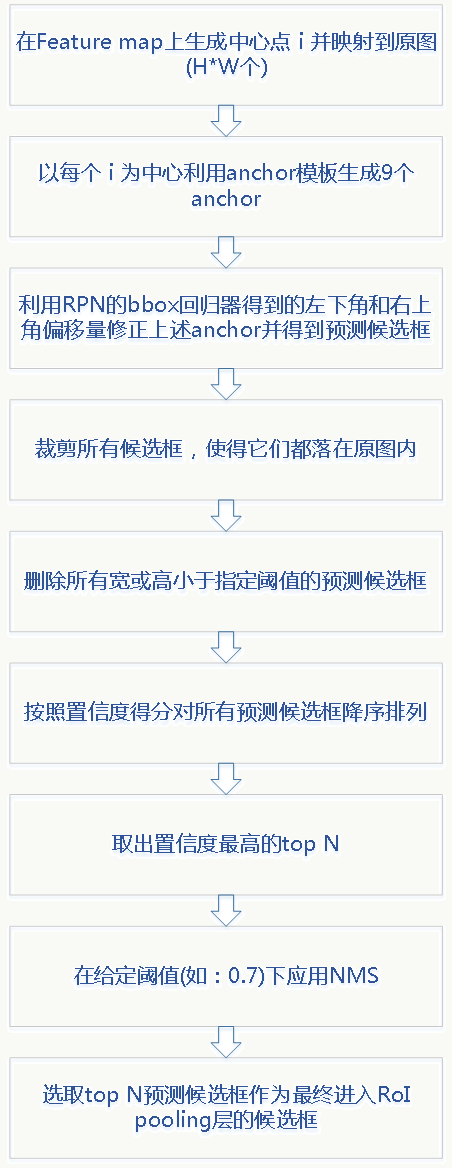
如上所述,Faster R-CNN设计了RPN使得候选框生成可以共用特征提取网络,算法流程如下: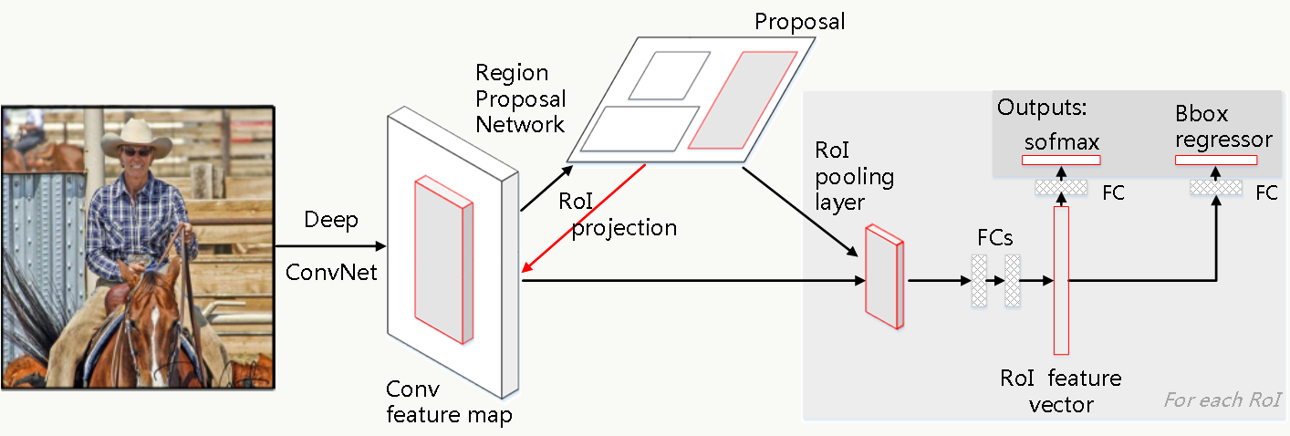
RPN负责生成Proposal候选框,其他过程类似Fast R-CNN,同样,生成候选框的扫描过程发生在最后一个卷积层产生的feature map上(而不是扫描原图),通过之前讲的坐标换算关系可以将feature map任意一点映射回原图。
8.6.2 RPN
RPN的结构如下: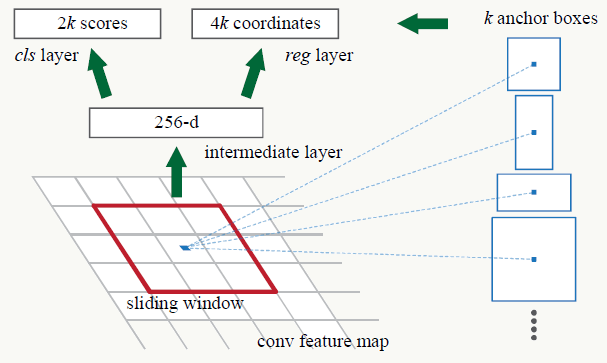
1、RPN的输入是特征提取器最后一个卷积(pooling)产生的feature map,例如VGG16为conv5_3产生的512维(channel数)的feature map(图中例子是256维);
2、之后以m×m大小的滑动窗口扫描feature map,如果feature map大小为h×w,则扫描h×w次(即以每个像素点为中心做一次),文中m的取值为3,取值与具体网络结构有关,感受野的不同导致候选框的初始大小不同;
3、每做一次滑动窗口会生成k个初始候选框,初始候选框的大小与anchor(原理8.6.3解释)有关,中心点为滑动窗口中心点,即对一次滑动窗口行为,所有利用anchor生成的候选框都有相同的中心点(图中蓝点),一定注意:这里的anchor及利用它生成的候选框都是相对于原图的位置;
4、定义两个分支,第一个分支(左边)是一个二分类器,用来区分当前候选框是否为物体,如果有k个由anchor生成的候选框,则输出2k个值(2维向量为:[是物体的概率,是背景的概率]);第二个分支(右边)为回归器,用来回归候选框的中心点坐标和宽与高(4维向量[x,y,w,h]),如果有k个由anchor生成的候选框,则输出4k个值,显然这里候选框的生成要短、平、快,精调细选由后续网络来做。
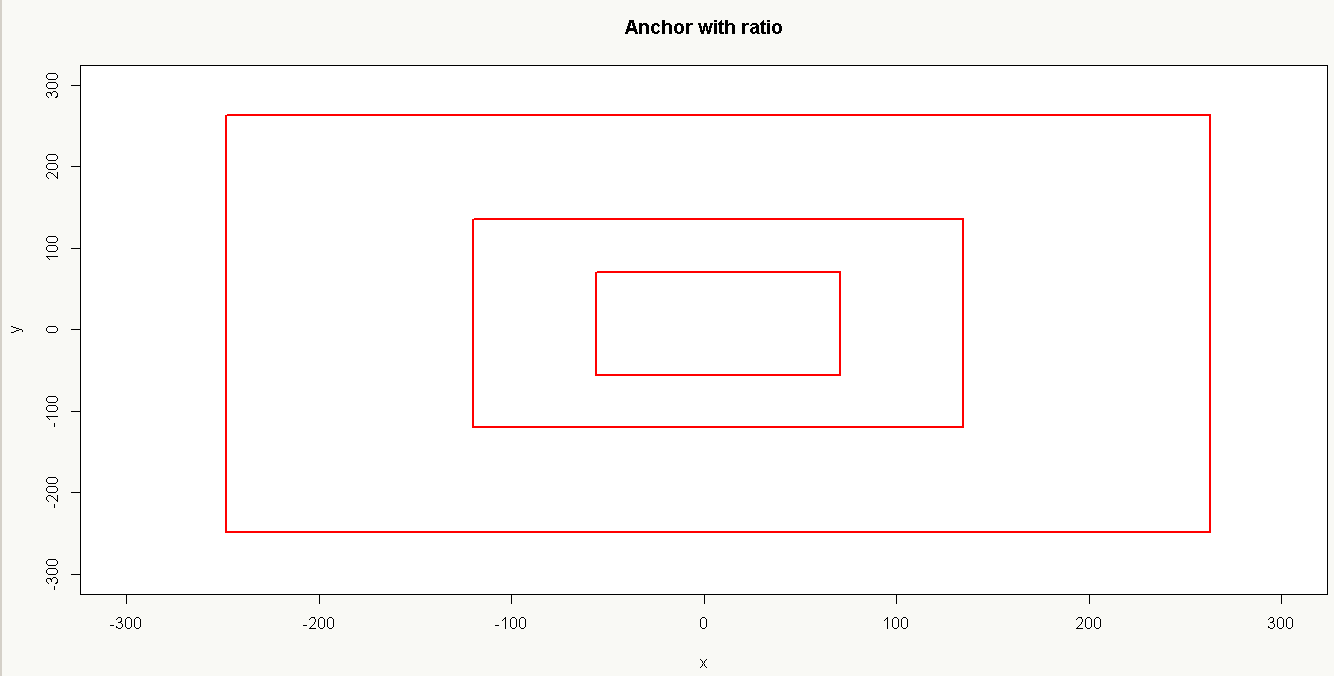
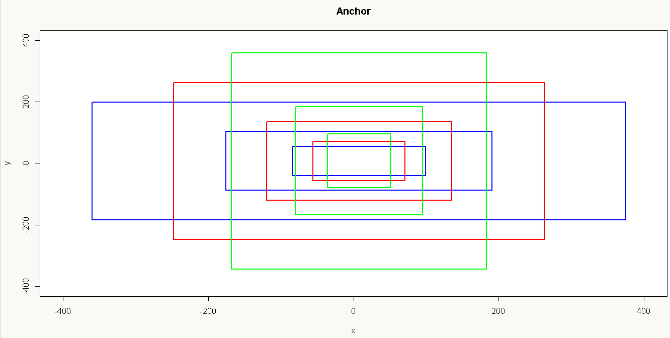
8.6.3 Anchor
RPN里很重要的一个概念是anchor,可以把它理解为生成候选框的模板,在RPN里只生成一次,anchor是用原图为参照物,以(0,0,指定宽,指定高)四元组采用不同缩放比例和尺度后产生的候选框模板集合,而候选框由滑动窗口(中心点x,中心点y)利用anchor生成。也可以从逆SPP角度去理解,SPP可以把一个feature map通过多尺度变换为金字塔式的多个feature map,反过来任何一个feature map也可利用多尺度变成多个feature map,这么做的好处是压根儿不用在原图上做各种尺度缩放而只用在feature map上做就好,并且这种变换具有不变性(Translation-Invariant Anchor):候选框生成及其预测函数具有可复现性,例如通过k-means聚类得到800个anchor,如果重复做一次实验不一定还是原来那800个,这个性质可以降低模型大小以及过拟合的风险。
以16×16大小为,base anchor[0,0,15,15]为例:
1、只使用_ratio_enum生成候选框如下: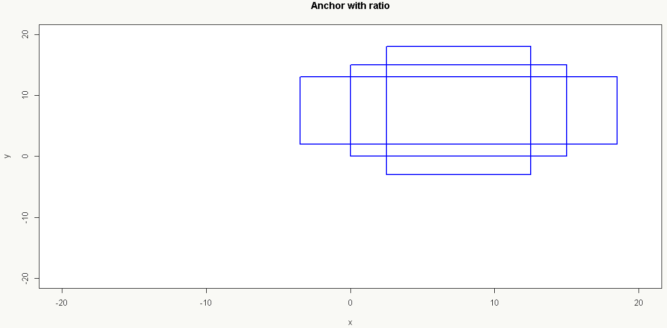
代码可参考generate_anchors.py:
1 | # -------------------------------------------------------- |
8.6.4 代码实践
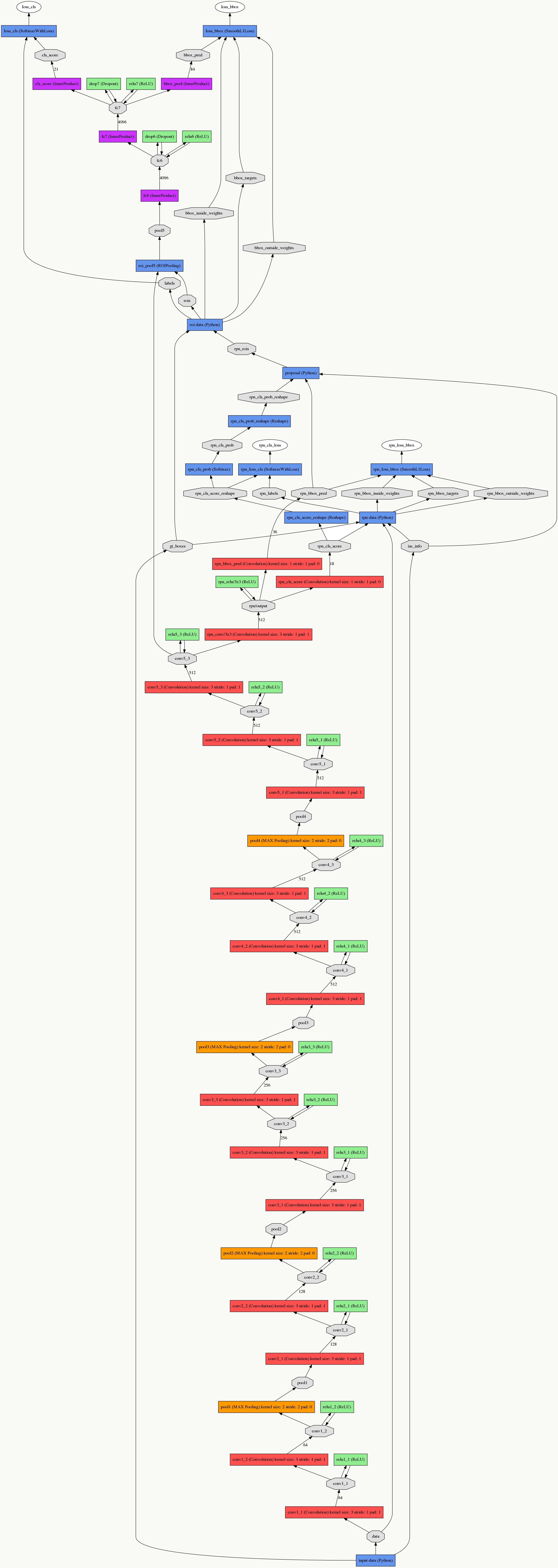
集中介绍RPN中proposal层的实现,以特征提取网络采用VGG16在poscal_voc数据集上为例。
网络结构
![]()
RPN配置
1
2
3
4
5
6
7
8
9
10
11
12
13
14
15
16
17
18
19
20
21
22
23
24
25
26
27
28
29
30
31
32
33
34
35
36
37
38
39
40
41
42
43
44
45
46
47
48
49
50
51
52
53
54
55
56
57
58
59
60
61
62
63
64
65
66
67
68
69
70
71
72
73
74
75
76
77
78
79
80
81
82
83
84
85
86
87
88
89
90
91
92
93
94
95
96
97
98
99
100
101
102
103layer {
name: "rpn_conv/3x3"
type: "Convolution"
bottom: "conv5_3"
top: "rpn/output"
param { lr_mult: 1.0 }
param { lr_mult: 2.0 }
convolution_param {
num_output: 512
kernel_size: 3 pad: 1 stride: 1
weight_filler { type: "gaussian" std: 0.01 }
bias_filler { type: "constant" value: 0 }
}
}
layer {
name: "rpn_relu/3x3"
type: "ReLU"
bottom: "rpn/output"
top: "rpn/output"
}
layer {
name: "rpn_cls_score"
type: "Convolution"
bottom: "rpn/output"
top: "rpn_cls_score"
param { lr_mult: 1.0 }
param { lr_mult: 2.0 }
convolution_param {
num_output: 18 # 2(bg/fg) * 9(anchors)
kernel_size: 1 pad: 0 stride: 1
weight_filler { type: "gaussian" std: 0.01 }
bias_filler { type: "constant" value: 0 }
}
}
layer {
name: "rpn_bbox_pred"
type: "Convolution"
bottom: "rpn/output"
top: "rpn_bbox_pred"
param { lr_mult: 1.0 }
param { lr_mult: 2.0 }
convolution_param {
num_output: 36 # 4 * 9(anchors)
kernel_size: 1 pad: 0 stride: 1
weight_filler { type: "gaussian" std: 0.01 }
bias_filler { type: "constant" value: 0 }
}
}
layer {
bottom: "rpn_cls_score"
top: "rpn_cls_score_reshape"
name: "rpn_cls_score_reshape"
type: "Reshape"
reshape_param { shape { dim: 0 dim: 2 dim: -1 dim: 0 } }
}
layer {
name: 'rpn-data'
type: 'Python'
bottom: 'rpn_cls_score'
bottom: 'gt_boxes'
bottom: 'im_info'
bottom: 'data'
top: 'rpn_labels'
top: 'rpn_bbox_targets'
top: 'rpn_bbox_inside_weights'
top: 'rpn_bbox_outside_weights'
python_param {
module: 'rpn.anchor_target_layer'
layer: 'AnchorTargetLayer'
param_str: "'feat_stride': 16"
}
}
layer {
name: "rpn_loss_cls"
type: "SoftmaxWithLoss"
bottom: "rpn_cls_score_reshape"
bottom: "rpn_labels"
propagate_down: 1
propagate_down: 0
top: "rpn_cls_loss"
loss_weight: 1
loss_param {
ignore_label: -1
normalize: true
}
}
layer {
name: "rpn_loss_bbox"
type: "SmoothL1Loss"
bottom: "rpn_bbox_pred"
bottom: "rpn_bbox_targets"
bottom: 'rpn_bbox_inside_weights'
bottom: 'rpn_bbox_outside_weights'
top: "rpn_loss_bbox"
loss_weight: 1
smooth_l1_loss_param { sigma: 3.0 }
}准备阶段 配置参数和生成anchor模板:
1
2
3
4
5
6
7
8
9
10
11
12
13
14
15
16
17
18
19
20
21
22
23
24
25
26def setup(self, bottom, top):
# parse the layer parameter string, which must be valid YAML
layer_params = yaml.load(self.param_str_)
# 获取所有特征提取层stride的乘积。(例如VGG为16)
self._feat_stride = layer_params['feat_stride']
# 设置初始尺度变换比例为8、16、32。
anchor_scales = layer_params.get('scales', (8, 16, 32))
# 使用上面介绍的方法生成anchor模板。
self._anchors = generate_anchors(scales=np.array(anchor_scales))
# anchor数量。(例如:9)
self._num_anchors = self._anchors.shape[0]
if DEBUG:
print 'feat_stride: {}'.format(self._feat_stride)
print 'anchors:'
print self._anchors
# rois blob: holds R regions of interest, each is a 5-tuple
# (n, x1, y1, x2, y2) specifying an image batch index n and a
# rectangle (x1, y1, x2, y2)
top[0].reshape(1, 5)
# scores blob: holds scores for R regions of interest
if len(top) > 1:
top[1].reshape(1, 1, 1, 1)前向传播
![]()

实现上就是中心点i的各个坐标直接加到anchor模板的各个坐标即可(anchor模板是以0为中心点的),代码类似:
1 | A = self._num_anchors |
8.6.5 Faster R-CNN训练流程
采用四阶段交替方式训练(4-Step Alternating Training)
1、使用ImageNet预训练模型权重初始化并fine-tuned训练一个RPN;
2、使用ImageNet预训练模型权重初始化并将上一步产生的候选框(proposal)作为输入训练独立的Faster R-CNN检测模型(此时没有卷积网络共享);
3、生成新的RPN并使用上一步Fast-RCNN模型参数初始化,设置RPN、Fast-RCNN共享的那部分网络权重不做更新,只fine-tuned训练RPN独有的网络层,达到两者共享用于提取特征的卷积层的目的;
4、固定共享的那些卷积层权重,只训练Fast-RCNN独有的网络层。
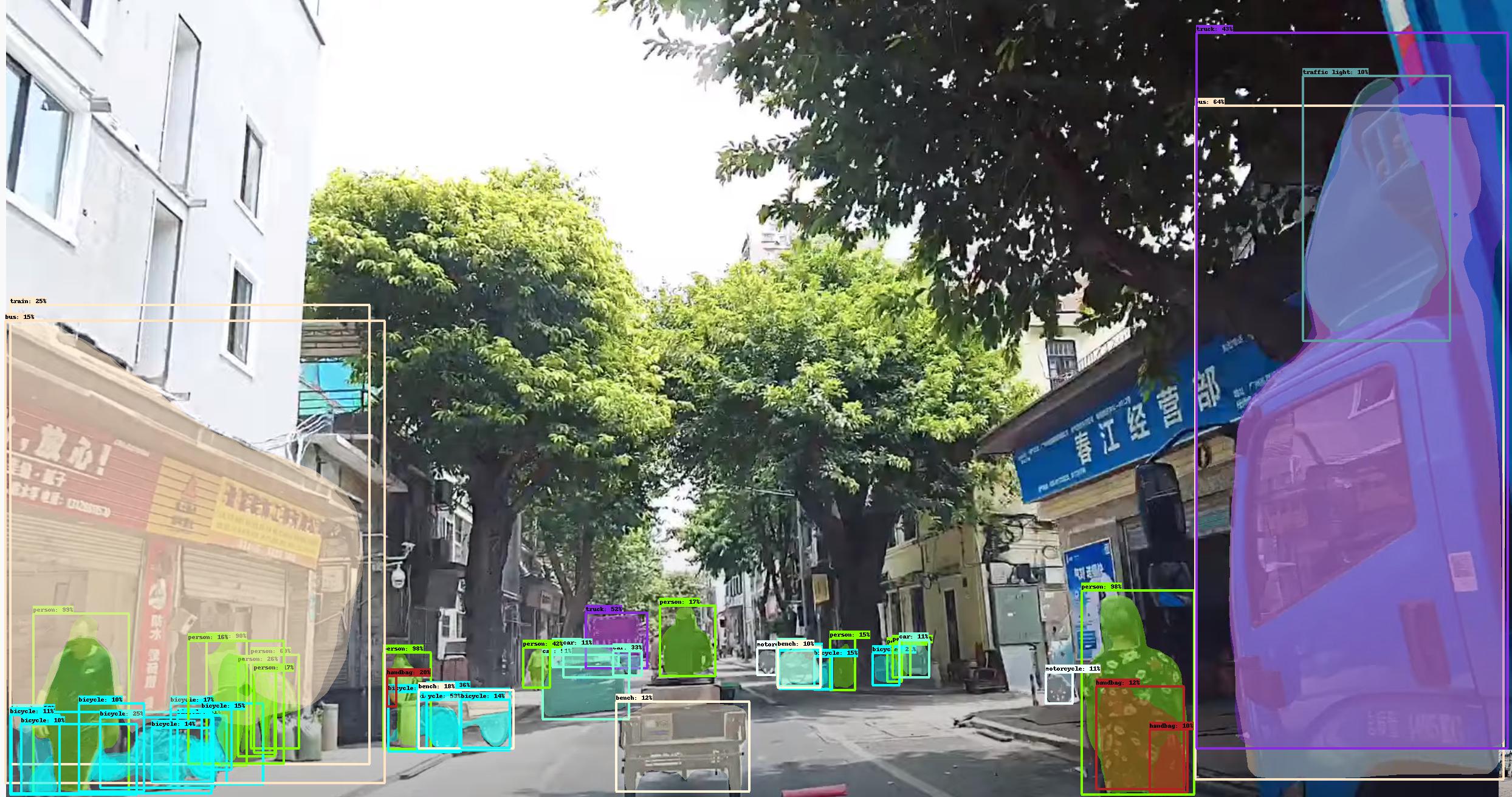
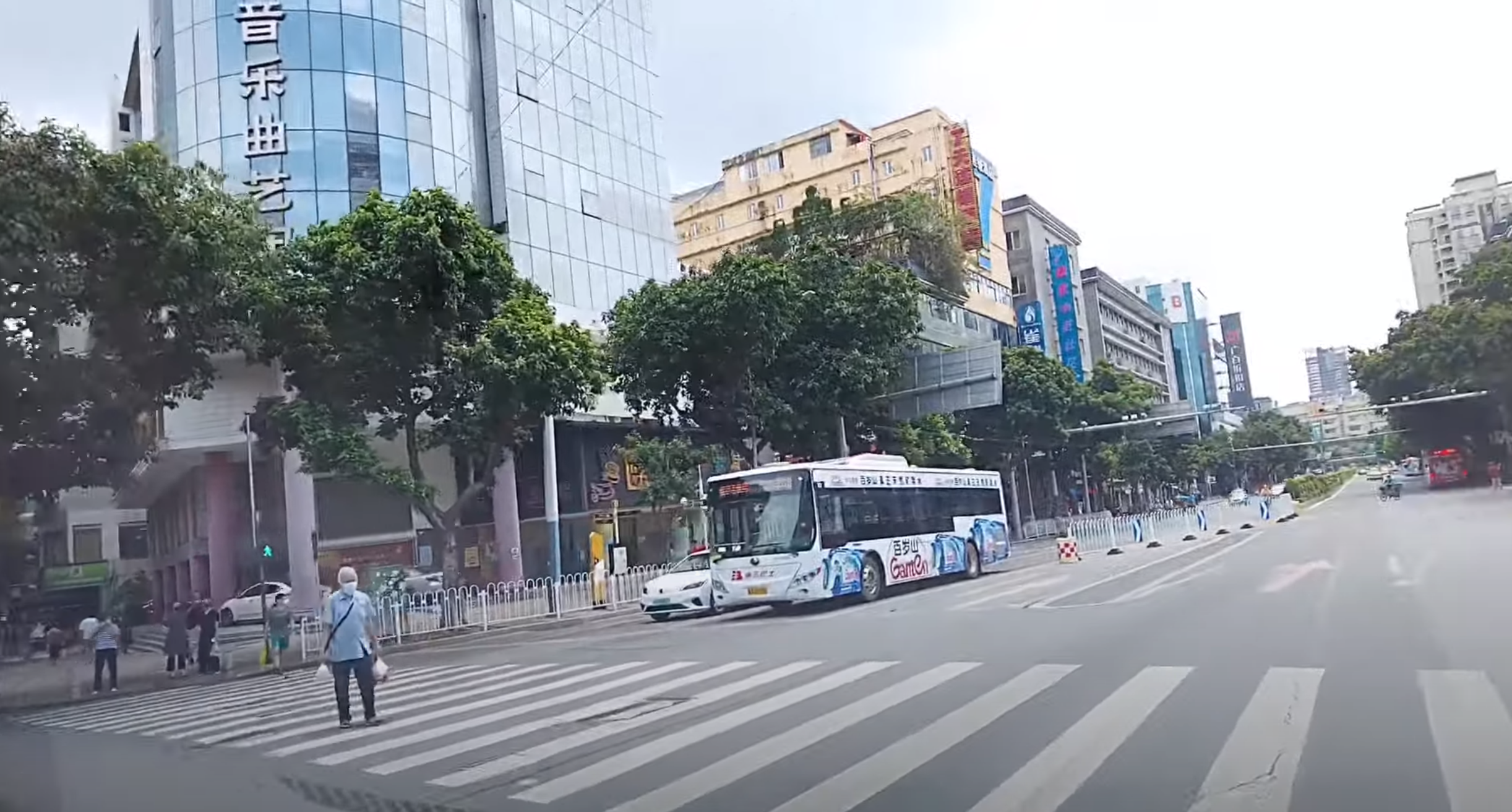
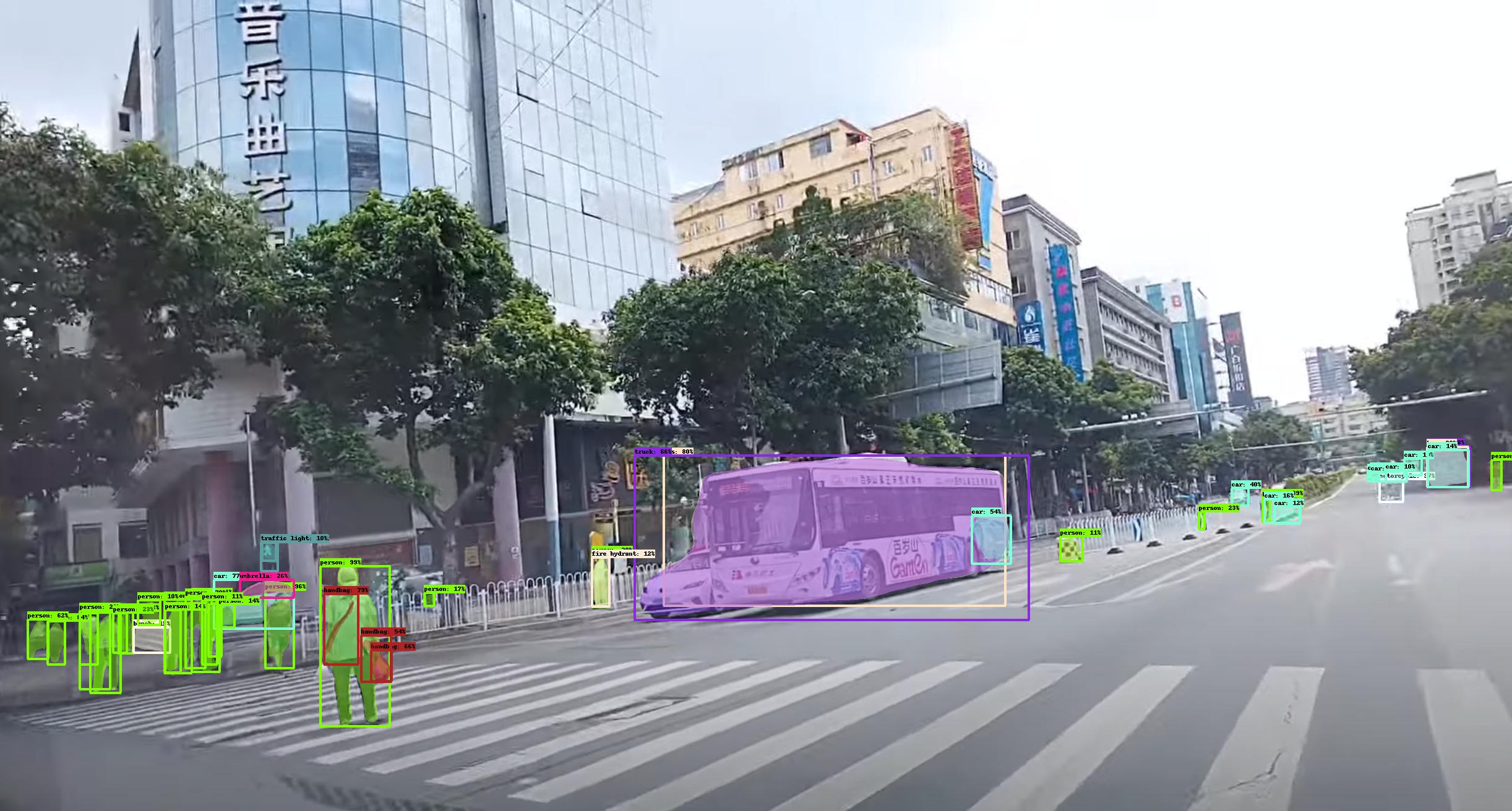
Faster R-CNN是效果最好的目标检测与分类模型之一,但如果想用于实时监测和前置到客户端则需要做大量模型裁剪、压缩和优化工作,具体做法我以后介绍,目前我们做的比较初步,模型大小压缩到10m左右,准确率损失小于1.5%,线上inference响应时间在500k左右大小图片、k80单机单卡单次请求下为20ms左右(在高并发情况下会通过打batch的方式及其他方法提高并发量)。
未做优化的汽车检测demo: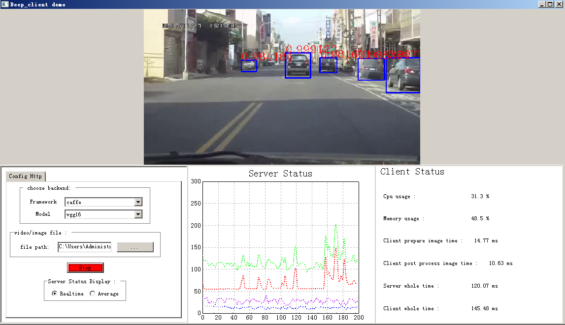
8.6.6 Faster R-CNN with Caffe
源码地址:Faster R-CNN(rbgirshick版)。 一定注意,caffe有个问题(我认为是架构上的设计缺陷,这个问题tensorflow就没有):由于要支持自定义的网络层之类的需求,每个人的caffe版本可能是不一样的,所以在编译时需要注意,比如这里的caffe必须使用0dcd397这个branch,否则编译不通过,因为这里有自定义的proposal层以及相关参数。 目录结构如下: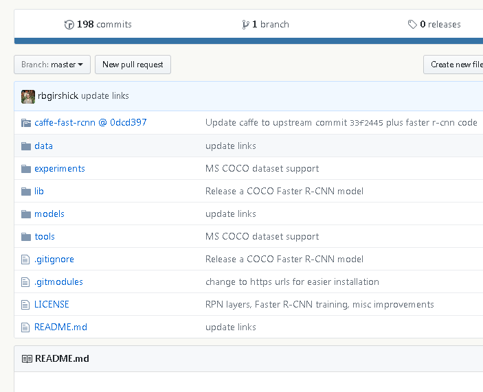
Centos 7上编译运行caffe及Faster R-CNN
编译准备 1、 为你的账号添加sudo权限
2、安装编译器1
gpasswd -a user_name wheel
3、安装 git1
sudo yum install gcc gcc-c++
4、clone代码1
sudo yum install git
5、安装依赖项1
git clone https://github.com/rbgirshick/py-faster-rcnn.git
6、安装cmake1
sudo yum install snappy-devel opencv-devel atlas-devel boost-devel protobuf-devel
7、安装automake1
sudo yum install cmake
8、安装gflags1
2
3
4
5
6wget http://ftp.gnu.org/gnu/automake/automake-1.14.tar.gz
tar -xvf automake-1.14.tar.gz
cd automake-1.14
./configure
make -j
sudo make install9、安装glog1
2
3
4
5
6
7
8
9
10
11git clone https://github.com/gflags/gflags
cd gflags
mkdir build && cd build
export CXXFLAGS="-fPIC" && cmake ..
make VERBOSE=1 -j
sudo make install10、安装 lmdb1
2
3
4
5git clone https://github.com/google/glog
cd glog
./autogen.sh && ./configure && make && make install11、安装 hdf51
2
3
4
5
6
7git clone https://github.com/LMDB/lmdb
cd lmdb/libraries/liblmdb
make -j
sudo make install1
2
3
4
5
6
7
8
9
10
11wget https://support.hdfgroup.org/ftp/HDF5/current18/src/hdf5-1.8.19.tar.gz
tar -xvf hdf5-1.8.19.tar.gz
cd hdf5-1.8.19
./configure --prefix=/usr/local
make -j
sudo make install12、安装 leveldb
1
2
3
4
5
6
7
8
9
10
11git clone https://github.com/google/leveldb
cd leveldb
make -j
sudo cp out-shared/libleveldb.so* /usr/local/lib
sudo cp out-static/*.a /usr/local/lib
sudo cp -r include/* /usr/local/include编译caffe
1、下载源码
1
2cd py-faster-rcnn
git clone https://github.com/rbgirshick/caffe-fast-rcnn.git检查文件/src/caffe/proto/caffe.proto是否与下面文件一致: 点击下载 caffe.proto 文件
2、修改配置
修改它的几个地方:1
2
3
4
5cd caffe-fast-rcnn
cp Makefile.config.example Makefile.config
vim Makefile.config1)、指定CUDA_DIR,如:CUDA_DIR := /usr/local/cuda 2)、BLAS := open 3)、WITH_PYTHON_LAYER := 13、编译caffe-fast-rcnn
4、编译py-faster-rcnn的lib1
2
3
4
5
6
7
8
9make clean
make all -j
make test -j
make runtest -j
make pycaffe -j5、配置环境变量1
2
3cd py-faster-rcnn/lib/
make1
2
3
4
5vim ~/.bashrc
export PYTHONPATH=/data/liyiran/py-R-FCN/tools/python:$PYTHONPATH
source ~/.bashrc运行示例
1、下载pascal_voc数据集
2、下载预训练模型1
2
3
4
5
6
7cd py-faster-rcnn/data
wget http://host.robots.ox.ac.uk/pascal/VOC/voc2007/VOCtrainval_06-Nov-2007.tar
tar -xvf VOCtrainval_06-Nov-2007.tar
mv VOCtrainval_06-Nov-2007 VOCdevkit20071
2
3cd py-faster-rcnn/model
wget https://dl.dropboxusercontent.com/s/gstw7122padlf0l/imagenet_models.tgz?dl=03、使用VGG16,应用于pascal_voc 2007数据集
1
sh experiments/scripts/faster_rcnn_end2end.sh 1 VGG16 pascal_voc
8.7 R-FCN
回想之前所有基于Region的检测算法,有一个共同点是:整个网络被分成两部分:共享计算的、与Region无关的全卷积子网络和RoI Pooling之后不共享计算的、与Region相关的子网络(如RPN和BBox Regression网络)。再回想之前所有的分类网络,尤其到残差和GoogLeNet系列,都可以看做是全卷积网络,且在分类问题上的效果已经非常赞了,但当把这些网络直接用于检测问题时,效果往往特别差,甚至不如VGG-16,原因也是明确的:分类问题往往会忽略位置信息,只需要判断是否为某个物体,所以要求提取出来的特征具有平移不变性,不管图片特征放大、缩小还是位移都能很好的适应,而卷积操作、pooling操作都能较好的保持这个性质,并且网络越深模型越对位置不敏感;但在检测问题中,提取的特征还需要能敏锐的捕捉到位置信息,即具备平移变化性,这就尴尬了。为此,大家插入类似RoI Pooling这样的层结构,一方面是的任意大小图片都可以输入,更重要的是一定程度上弥补了位置信息的缺失,所以检测效果也就嗖嗖的上来了。但带来一个副作用是:RoI后每个Region都需要跑一遍后续子网络,计算不共享就导致训练和Inference的速度慢,为此代季峰、何凯明几位提出《R-FCN: Object Detection via Region-based Fully Convolutional Networks》检测框架,用Position-Sensitive RoI Pooling代替原来的RoI Pooling,共享了所有计算,很好的tradeoff了平移不变性和平移变化性,并且由于是全卷积,训练和Inference的速度更快。
以ResNet-101为例,图片来源: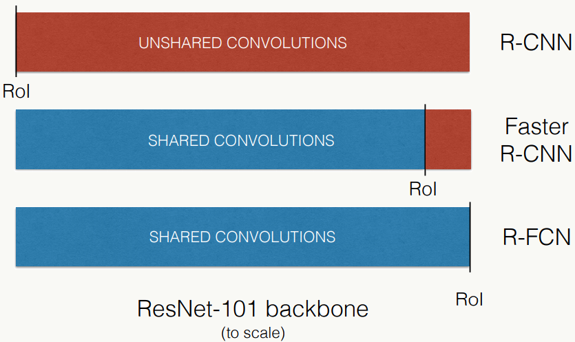
8.7.1 算法概述
1、核心思想
如上所述,算法核心就是position-sentitive RoI pooling的加入,核心思想是这样的: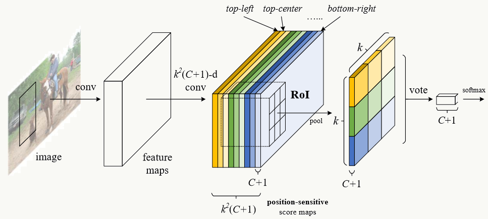
这里的feature map是过去RoI Pooling前的全卷积特征提取子网络,之后接着的(彩色立方体)是position-sensitive feature map,它其实是一个普通的卷积层,权重通过position-sensitive RoI Pooling层反向传播时修正。假设position-sensitive feature map(后面简写为ps feature map)的大小为k×k,检测分类数为C+1(1为背景类),则ps feature map的通道数为:k×k×(C+1),假如K=3,则每一类的 ps feature map会有k×k=9个,每个feature map含有一类位置特征(如:左上、左中、左右、......,下右,图中用不同颜色代表);接着,通过ps RoI Pooling后,每个RoI Region在C+1的每一类上都会得到一个k×k网格,对每个网格做分类判断,之后所有网格一起投票。最终得到C+1维向量,然后接个softmax做分类。
2、整体结构
考虑RPN子网络,整体结构是这样的:
对RPN来说也是类似,每个Bounding Box候选框的位置为一类(左上角坐标、长和宽),ps feature map的通道数为k×k×4。
3、position-sensitive feature map
以ResNet-101作为基础网络结构为例,做以下结构上的更改:
- 去掉GAP层和所有fc层
- 保留前100层,最后一个卷积层后接一个(1×1)×1024卷积层做降维
为了显示编码位置信息,假如ps feature map网格大小k×k,RoI大小为:\(w×h\),则每个bin大小约为:\(\frac{w}{k} ×\frac{h}{k}\),对于第(i,j)个bin(\(0\leq i,j\leq k-1\))做ps RoI Pooling为:
\[ r_c(i,j|\Theta)=\sum_{(x,y)\in bin(i,j)}z_{i,j,c}(x+x_0,y+y_0|\Theta)/n. \]
其中:
\(r_c(i,j)\)为第c类在第(i,j)个bin的pooling响应值;
\(z_{i,j,c}\)为是k×k×(C+1)个feature map中的一个;
\((x_0,y_0)\)为RoI的左上角坐标;
\(n\)是当前bin中的像素数;
\(\Theta\)是网络所有可学习参数;
x、y的取值范围为:\(\lfloor i\frac{w}{k}\rfloor \leq x \leq \lceil(i+1)\frac{w}{k}\rceil\),\(\lfloor j\frac{h}{k}\rfloor \leq y \leq \lceil(j+1)\frac{h}{k}\rceil\);
pooling采用average、max甚至其他自定义的操作。
4、损失函数定义
由分类部分和回归部分损失组成:
\[ L(s,t_{x,y,w,h})=L_{cls}(s_{c^*})+\lambda [c^*>0]L_{reg}(t,t^*) \] 其中:
\(c^*\)是每一类的label,\(c^*=0\)代表背景类;
\(L_{cls}(s_{c^*})=-log(s_{c^*})=-log(\frac{e^{r_{c^*}(\Theta)}}{\sum_{c=0}^{C}e^{r_{c(\Theta)}}})\),是交叉熵损失函数;
\(L_{reg}(t,t^*)=\sum_{i \in \{x,y,w,h\}}smooth_{L_1}(t-t^*)\),与Fast R-CNN的定义一致;
\([c^*>0] = \begin{cases}1& \text{if }c^*>0\\0& \text{otherwise}\end{cases}\)
5、可视化效果
预测正例: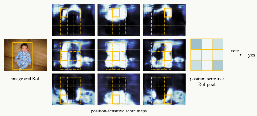
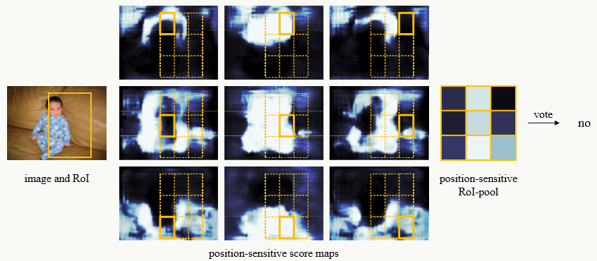
8.7.2 position-sentitive RoI pooling
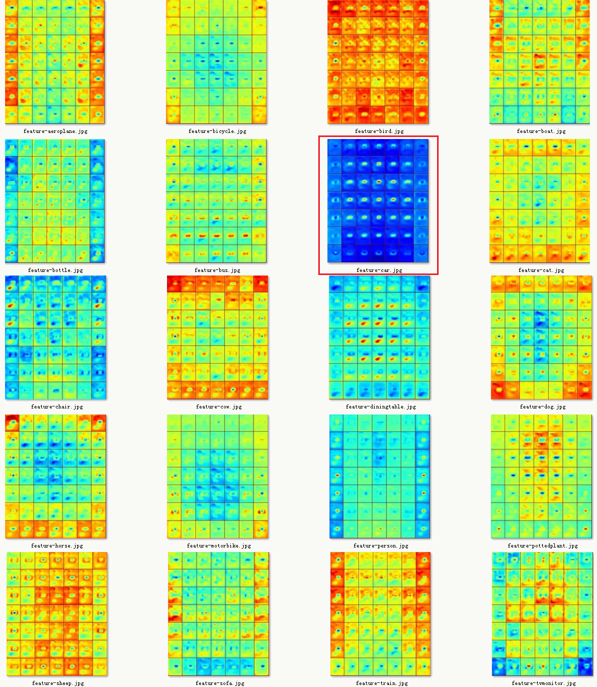
- 原图及检测图
- 所有分类下的位置敏感特征图
![]()
8.7.3 模型训练
1、训练使用Online Hard Example Mining
OHEM是一种boosting策略,目的是使得训练更加高效,简单说,它不是使用简单的抽样策略,而是对容易判断的样本做抑制,对模型不容易判断的样本重复添加。 在检测中,正样本定义为:与ground-truth的\(IoU\geq0.5\),反之为负样本,应用过程为:
- 前向传播:所有候选框在Inference后做损失排序,选取B(一共N个)个损失最高的候选框,当然,由于临近位置的候选框的损失相近,所以还需要对其做NMS(如取IoU=0.7),然后再选出这B个样本;
- 反向传播:仅用这B个样本做反向传播更新权重。
2、训练参数
- 权重衰减系数:0.0005
- 动量项取值:0.9
- 图像被缩放为600像素
- 每个GPU使用一张图像,选择B=128个候选框做反向传播
- 利用VOC数据做fine-tune
- 采用 Faster R-CNN的四步交替法训练
8.7.4 代码实践
源码可在py-R-FCN下载,需要把下载R-FCN版本caffe,编译方式类似Faster RCNN,目录类似:
- PSROIPooling
1 | // ------------------------------------------------------------------ |
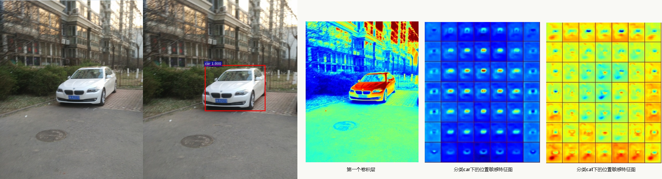
- PS feature map可视化
1 | #!/usr/bin/env python |
8.8 DenseNet
8.8.1 关于神经网络的深度
理论上,当我们有足够大量的数据,能够完全体现当前问题的数据分布的时候,我们仅需要一个简单线性模型或最多用个有单隐层的RBF神经网络就可以完美建模。但实际情况是没有那么多数据,那就自然需要一个高复杂度的模型来拟合样本,但如果模型复杂度过高而样本数没有与其达到某种关系,又会造成其泛化性低下,所谓过拟合的问题。实际上,假设未来做testing的数据分布和training的数据分布是一致的,一个有\(N\)个神经网络节点、\(W\)个权重、线性阈值函数的前馈神经网络在泛化误差\(0<\epsilon \le0.125\)的前提下,训练数据规模的下界是:\(m\ge O(\frac{W}{\epsilon}log\frac{N}{\epsilon})\),详情可见论文《What Size Net Gives Valid Generalization》。
网络的深度则反映了模型的复杂度,深度直接决定了层数而间接影响了节点数和权重数,网络深度的增加意味着能得到更多的抽象特征,但原始输入信号和梯度信息会随着网络深度的增加而消失或无用,所以这又是一个折中权衡,像之前讲的Highway Network、ResNet及其衍生等等模型的思路是通过一个short path的连接让前一层的信号能够传递到后一层,我认为这个思路是开创性的。
8.8.2 DenseNet思路
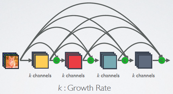
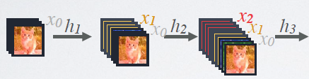
《Densely Connected Convolutional Networks》(CVPR 2017的最佳论文之一)提出的DenseNet则把ResNet的思路做的更加彻底:在一个Dense Block中,任意一个当前层都会与其后面的所有层直接连接,如图: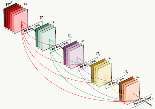
假如包括当前层在内后面还有\(L\)层,那么从当前层往后产生的直接连接数为:\(\frac{L(L+1)}{2}\)。
回顾之前对ResNet的分析以及《Deep Networks with Stochastic Depth》这篇论文的实验,可以得到以下信息:
神经网络不一定非得是逐层递进的,任意一层可以接收它前面任意一层的输入而扔掉它前面的其它层,也就是说当前层feature map的提取可以只依赖更前面层的feature map;
传统前馈神经网络架构可以被看做是有个状态维护机制,在层与层之间传递这个状态,后一层在接收前一层的状态后又加入自己的信息,修改状态后传给下一层;
ResNet网络在路径选择的思想下展开(见ResNet一章的分析)后,其实也说明它有一定的冗余性,适当的随机Dropout一些层相当于扔掉了一些路径,实际实验看还会提高网络Inference的泛化性。基于以上认知,作者设计了DenseNet:让每一层都与后面所有层直接连接,达到特征复用的目的;同时这些连接也可以看做网络的全局状态,大家共同维护,不用传来传去;降低每一层feature map数,让网络结构变“窄”,达到去除冗余的目的。
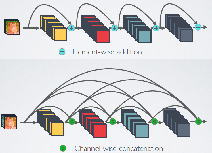
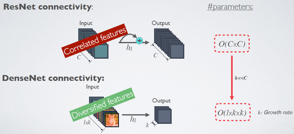
与ResNet比较:
ResNet采用按照向量每个维度的Element-wise做加和的方式处理连接,而DenseNet采用按照每个通道的Channel-wise做直接向量拼接的方式处理连接。
![]()
PS:注意图中C操作符的位置
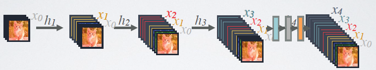
DenseNet的前向传播过程可以像这样展开:
![]()
每一层的输入都包含所有前面层的feature map。
形式化的对比如下:
ResNet:第\(l\)层的输出是\(x_l=H_l(x_{l-1})+x_{l-1}\)
DenseNet:第\(l\)层的输出是\(x_l=H_l([x_0,x_1,...,x_{l-1}])\)
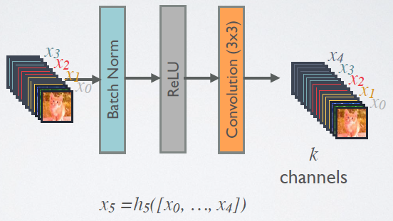
其中:\([]\)为向量拼接操作,\(H_l\)是一个复合函数,文中是batch normalization (BN)+rectified linear unit (ReLU)+3×3 convolution (Conv)的复合——BN(ReLU(Conv(x)))。
![]()
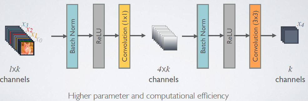
dense blocks与transition layer DenseNet的拼接操作要求保证feature map大小具有一致性,但由于pooling下采样操作的存在一定会改变feature map的,所以作者用dense blocks+transition layers的方式解决问题:
1、dense blocks内部feature map大小都一致,借鉴Inception结构,利用bottleneck中的1×1卷积降低通道数,即 BN+ReLU+Conv(1x1)+BN+ReLU+Conv(3x3) 操作;
2、dense blocks之间增加transition layer,同样借鉴Inception结构,利用1×1卷积降低通道数,即BN+ReLU+Conv(1×1)+AvgPooling(2x2) 操作:
![]()
transition layer可以起到压缩模型的作用:假设dense block有\(m\)个feature map,我们让紧接着的transition layer产生\(\lfloor \theta m\rfloor\),这里\(0<\theta\le1\)为压缩系数。
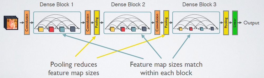
宏观来看,整个DenseNet如下:
![]()
利用Growth Rate和复合函数,DenseNet可以做的很“窄”:
![]()
假设每个\(H_l\)复合函数产生\(k\)个feature map,那么第\(l\)层的输入feature map数为:\(k_0+k\times(l-1)\) ,可见越往后的dense block输入feature map越多,当然由于全局feature map的存在,每层只有 \(k\) 个feature map是独有的,其余的都共享。 显然,“窄”的好处是参数少、计算效率高,比较如下:
![]()
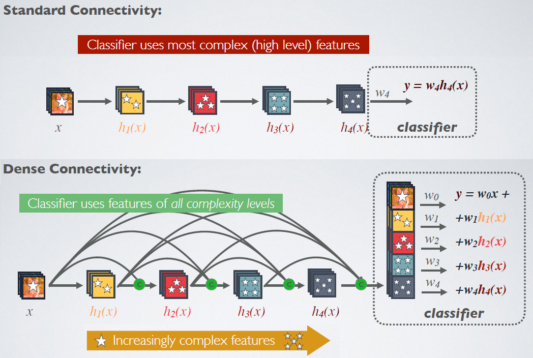
DenseNet结构使得特征更加具有多样性 显然,由于从高到低引入了不同复杂度的特征,使得最终做预测的特征具有很强的多样性,提高模型的泛化性和鲁棒性。
![]()
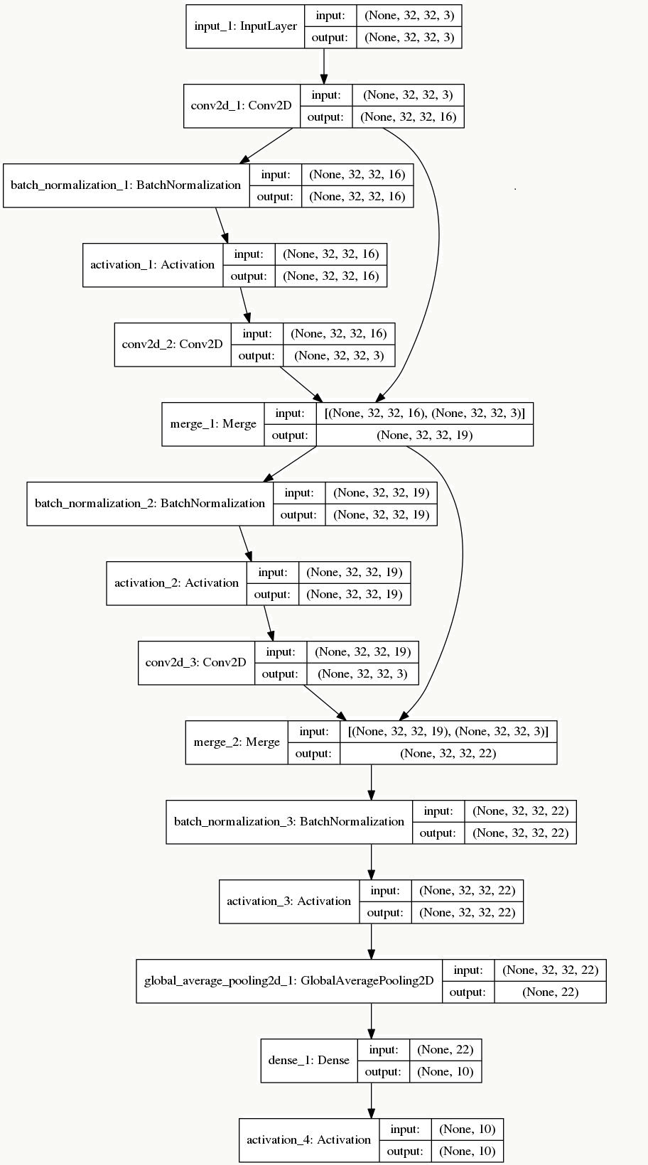
8.8.3 代码实践
看一个基于keras的简单例子,比较好重现了DenseNet的构建,看的时候对照着DenseNet的前向展开图更好理解原理:1 | # -*- coding: utf-8 -*- |
8.9 Mask R-CNN
8.9.1 算法概述
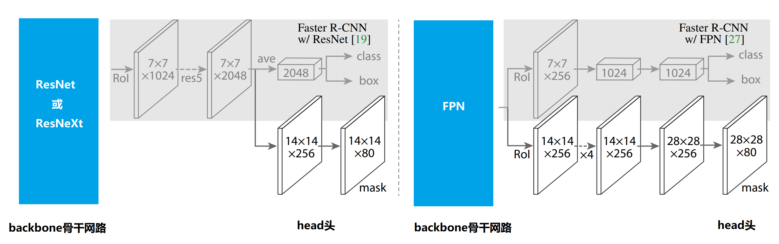
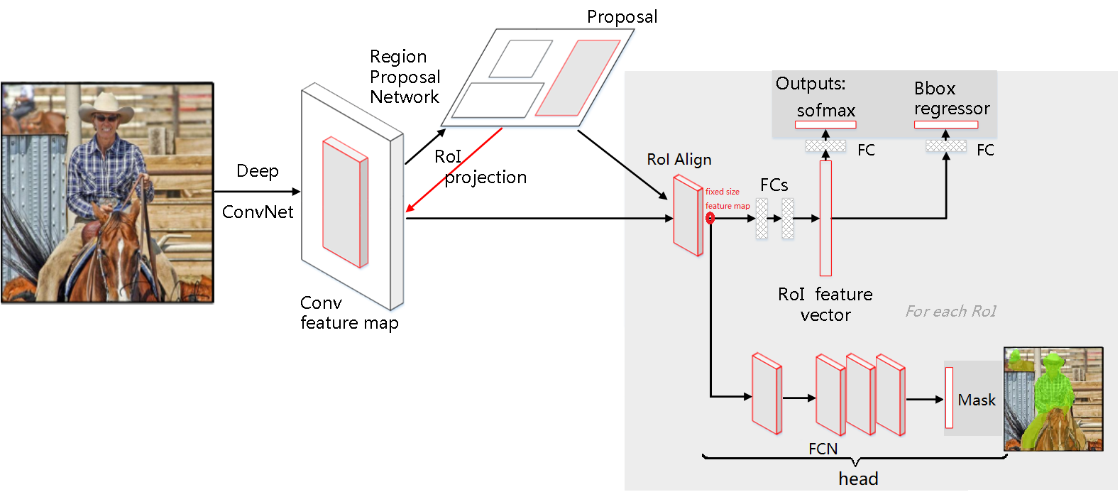
Mask R-CNN是何恺明等人在《Mask R-CNN》一文中提出的一个简单的、扩展性较强的用于目标检测、识别、实例和语义分割的通用框架,可以看做是Faster R-CNN的升级加强版,结构上也可以理解为:把原有Faster R-CNN的RoIPooling层替换为RoIAlign层,并加了第三个用来预测Mask的分支,以支持pixel2pixel像素粒度的分类预测(语义分割)。 演化过程如下:
8.9.2 Mask
需要注意的是,在Mask任务分枝下,假设有\(K\)个分类,则对每个RoI会针对所有\(K\)个分类产生一个\(m×m\)的binary masks(0或非0)预测图(即mask任务分支对每个RoI产生一个维度为\(Km^2\)的输出)。
由于这种像素级的分割对空间位置信息很敏感,而原有的RoI Pooling大量使用了取整操作(文中叫做harsh quantization),从而使得RoI Pooling的输出产生位移,会和原图像上的RoI对不上(ps:分类操作本就对位置不敏感,所以不受这种位移影响),所以文中采用了RoI Align来改进,使得提高了mask预测精度提高了10%到50%。 查看8.5 Fast R-CNN的代码介绍也可以发现,做原图到feature map的映射时用了round四舍五入以及计算bin在feature map上的坐标范围时用了floor取整操作。
1 | // rbgirshick/fast-rcnn对ROIPoolForward的实现: |
8.9.3 RoIAlign
图像的仿射变换 在图像处理中经常会用仿射变换去做各种图像处理,用数学表达为 : 假设,\(x,y\)是原始图像中某一点的位置,\(x^*,y^*\)是做了图像变换后该点的位置,则这个变换过程表示为: \[ \begin{bmatrix} x^* \\ y^* \end{bmatrix} =\begin{bmatrix} v_{11} & v_{12} & v_{13} \\ v_{21} & v_{22} & v_{23} \end{bmatrix} \cdot \begin{bmatrix} x \\ y \\ 1 \end{bmatrix} \] 假设有以下500×500图片:
![]()
以opencv中的仿射变换为例,常用的变换有:
变换 变换矩阵 例子 效果 恒等(Identity) \(\begin{bmatrix} 1 & 0 & 0 \\ 0 & 1 & 0 \end{bmatrix}\) \(\begin{bmatrix} 1 & 0 & 0 \\ 0 & 1 & 0 \end{bmatrix}\) ![]()
平移(Translation) \(\begin{bmatrix} 1 & 0 & v_{13}\geq 0 \\0 & 1 & v_{23}\geq 0 \end{bmatrix}\) \(\begin{bmatrix} 1 & 0 & 30 \\ 0 & 1 & 30 \end{bmatrix}\) ![]()
镜像(Reflection) \(\begin{bmatrix} -1 & 0 & v_{13}\geq 0 \\ 0 & 1 & 0 \end{bmatrix}\) \(\begin{bmatrix} -1 & 0 & 500 \\ 0 & 1 & 0 \end{bmatrix}\) ![]()
缩放(Scale) \(\begin{bmatrix} v_{11} & 0 & 0 \\ 0 & v_{22} & 0 \end{bmatrix}\) \(\begin{bmatrix} 1.5 & 0 & 0 \\ 0 & 1.5 & 0 \end{bmatrix}\) ![]()
旋转(Rotate) \(\begin{bmatrix} v_{11}=cos(\theta) & v_{12}=-sin(\theta) & 0 \\ v_{21}=sin(\theta) & v_{22}=cos(\theta) & 0 \end{bmatrix}\) \(\begin{bmatrix} 0.866 & -0.5 & 0 \\ 0.5 & 0.866 & 0 \end{bmatrix}_{\theta=\frac{\pi}{6}=30^\circ}\) ![]()
剪切(Shear) \(\begin{bmatrix} 1 & v_{12} & 0 \\ v_{21} &1 &0 \end{bmatrix}\) \(\begin{bmatrix} 1 & 0.5 & 0 \\ 0.5 & 1 & 0 \end{bmatrix}\) ![]()
代码如下:
1
2
3
4
5
6
7
8
9
10
11
12
13
14
15
16
17
18
19
20
21
22
23
24
25
26
27
28
29
30
31
32
33
34
35
36
37
38
39
40
41
42
43
44
45
46
47
48import cv2
import numpy as np
import matplotlib.pyplot as plt
def image_transformation(file_name, T):
img = cv2.imread(file_name)
new_img = cv2.warpAffine(img, T, img.shape[:2])
plt.figure(figsize=(50,50))
plt.subplot(121)
plt.imshow(img)
plt.xticks([])
plt.yticks([])
plt.subplot(122)
plt.imshow(new_img)
plt.xticks([])
plt.yticks([])
plt.show()
# 镜像
T1 = np.float32([[-1, 0, 500],
[0, 1, 0]])
# 恒等
T2 = np.float32([[1, 0, 0],
[0, 1, 0]])
# x和y同时平移平移
T3 = np.float32([[1, 0, 30],
[0, 1, 30]])
# 缩放
T4 = np.float32([[1.5, 0, 0],
[0, 1.5, 0]])
# 旋转
T5 = np.float32([[0.866, -0.5, 0],
[0.5, 0.866, 0]])
# 剪切
T6 = np.float32([[1, 0.5, 0],
[0.5, 1, 0]])
image_transformation('me.jpeg', T1)
image_transformation('me.jpeg', T2)
image_transformation('me.jpeg', T3)
image_transformation('me.jpeg', T4)
image_transformation('me.jpeg', T5)
image_transformation('me.jpeg', T6)线性插值 在要求没那么高的场景中,为了弥补相近两个数据中间缺失的数据,常常采用线性插值法,即假设两点之间的数据分布为线性分布,显然如果曲线曲率越大,线性插值的误差越大。 形式化表示如下:
![]()
假设:已知坐标 \((x_0, y_0)\) 和 \((x_1, y_1)\),要在两点间插入一点\((x,y)\)作为补充数据,其中\(x\)的值已指定,则\(y\)的值为: \[ \frac{y-y_0}{x-x_0}=\frac{y_1-y_0}{x_1-x_0} \] 得到: \[ \begin{align*} y&=y_0+\frac{x-x_0}{x_1-x_0}y_1-\frac{x-x_0}{x_1-x_0}y_0\\ &=\frac{x-x_0}{x_1-x_0}y_1+\frac{x_1-x}{x_1-x_0}y_0 \end{align*} \]
双线性插值 双线性插值是对线性插值在二维上的扩展,基本思想是利用某点周围的四个点估计出该点的值,形式化表示如下:
![]()
问题:想得到未知函数\(f\)在点\(P(x,y)\)的值。(以图像为例:已知图像上某个位置,想得到在这个位置的灰度值)
假设:已知函数\(f\)在\(P\)点 周围 四个点的函数值:\(Q_{11}=(x_1,y_1)\)、\(Q_{12}=(x_1,y_2)\)、\(Q_{21}=(x_2,y_1)\)、\(Q_{22}=(x_2,y_2)\)。(以图像为例:“周围隐含\(x_2-x_1=1\)且\(y_2-y_1=1\))
则:双线性插值会先在\(x\)轴方向做线性插值2次,后在\(y\)轴方向做线性插值1次,从而得到目标值。(ps:效果等同于在\(y\)轴方向插值2次,后在\(x\)轴方向插值1次) 即:在\(x\)轴方向做线性插值2次得到, \[ \begin{align*} f(R_1)=f(x,y_1)&=\frac{x_2-x}{x_2-x_1}f(Q_{11})+\frac{x-x_1}{x_2-x_1}f(Q_{21})\\ f(R_2)=f(x,y_2)&=\frac{x_2-x}{x_2-x_1}f(Q_{12})+\frac{x-x_1}{x_2-x_1}f(Q_{22}) \end{align*} \] 在\(y\)轴方向做线性插值1次得到, \[ \begin{align*} f(P)=f(x,y)&=\frac{y_2-y}{y_2-y_1}f(R_{1})+\frac{y-y_1}{y_2-y_1}f(R_{2})\\ &=\frac{y_2-y}{y_2-y_1}(\frac{x_2-x}{x_2-x_1}f(Q_{11})+\frac{x-x_1}{x_2-x_1}f(Q_{21}))+\frac{y-y_1}{y_2-y_1}(\frac{x_2-x}{x_2-x_1}f(Q_{12})+\frac{x-x_1}{x_2-x_1}f(Q_{22}))\\ &=\frac{1}{(x_2-x_1)(y_2-y_1)}(f(Q_{11})\underbrace{(x_2-x)(y_2-y)}_{w_{11}}+f(Q_{21})\underbrace{(x-x_1)(y_2-y)}_{w_{21}}+f(Q_{12})\underbrace{(x_2-x)(y-y_1)}_{w_{12}}+f(Q_{22})\underbrace{(x-x_1)(y-y_1)}_{w_{22}})\\ \end{align*} \]
细心的读者一定已经发现:插值后的\(P\)点取值也可以看做是周围4个点取值的线性加权之和,且权重:\(w_{11}+w_{21}+w_{12}+w_{22}=1\) 上式表达为矩阵形式为: \[ f(x,y)=\frac{1}{(x_2-x_1)(y_2-y_1)}\begin{bmatrix} x_2-x & x-x_1 \end{bmatrix}\cdot \begin{bmatrix} f(Q_{11}) & f(Q_{12}) \\ f(Q_{21}) & f(Q_{22}) \end{bmatrix} \cdot \begin{bmatrix} y_2-y \\ y-y_1 \end{bmatrix} \]
在图像矩阵上利用某点周围四个点的灰度值估计该点灰度值时,上式简化为矩阵形式: \[ f(P)=f(x,y)=\begin{bmatrix} x_1+1-x & x-x_1 \end{bmatrix}\cdot \begin{bmatrix} f(Q_{11}) & f(Q_{12}) \\ f(Q_{21}) & f(Q_{22}) \end{bmatrix} \cdot \begin{bmatrix} y_1+1-y \\ y-y_1 \end{bmatrix} \] 或等式: \[ f(x,y)=\sum_{i=1}^{2}\sum_{j=1}^{2}f(x_i,y_j)max(0,1-|x-x_i|)max(0,1-|y-y_i|)\tag{1} \]
RoIAlign 不管RoI Pooling还是RoI Align,都是为了把任意大小的RoI(注意这里不是bounding box)区域映射为相同固定大小的输出,前者由于量化误差的存在(四舍五入或取整),导致边界上的数据丢失,从而会使得RoI的边界从原图映射到Feature Map后出现偏离,如下图:
![]()
绿色为RoI映射后的理论边界,蓝色为实际边界
这种偏离对分类问题无影响(忽略精确的边界信息反而会提高分类准确率),但对语义分割确影响比较大(因为每个像素都要分类,所以精确的空间位置信息很重要),作者使用RoIAlign后可以使mask的精度提高10%~50%。 具体做法使用了:《Spatial Transformer Networks》一文介绍的双线性插值方法,如图:
![]()
基本过程如下:
1、保留边界,对边界不做量化操作,保持浮点数边界,并将RoI分为\(H×W\)(如3×3)的个子网格(Bin),每个子网格的边界也保留浮点数边界,即:我们不需要处理位置“坐标”,只需要处理“值”(相比较,RoIPooling做了两次量化:一次是原图映射到Feature Map时,一次是划分bin做Pooling时):
![]()
2、采样与插值,整体示意图如下:
![]()
每个Bin取4个规则的采样点,采样方法如下: \[ \begin{align*} x&=x_l+(i + 0.5)\frac{x_h-x_l}{n}\tag{2.1}\\ y&=y_l+(j + 0.5)\frac{y_h-y_l}{n}\tag{2.2}\\ n&=number \quad of \quad samples.\\ i,j&=0,...,n \end{align*} \] 对应上图中:\(x_l=min(x_1,x_2)\)、\(x_h=max(x_1,x_2)\)、\(y_l=min(y_1,y_2)\)、\(y_h=max(y_1,y_2)\),当\(n=2\)时,每个Bin采样后得到图中4个采样点(绿点)。
然后对每个采样点(以红点标注的那个采样点\(P\)点为例)取周围4个点得到2×2个子区域,取每个子区域的中点(途中黑色的\(Q_{11}、Q_{12}、Q_{21}、Q_{22}\)点)做双线性插值,得到该采样点\(P\)处的值。
![]()
原理及细节说明 上面的描述比较抽象,现在我们看个例子帮助大家理解: 1、假设输入原图为512×512,以stride=32,产生的feature map为16×16,每个RoI会被处理输出为一个固定大小的3×3的feature map:
![]()
2、以图中最下方的RoI为示例对象,假设其最左上角坐标为:\((5.26, 9.33)\),\(width=\frac{200}{32}=6.25\),\(height=\frac{185}{32}=5.78\),如下图:
![]()
3、显然边界坐标都不是整数,传统的RoI Pooling会做量化,把边界信息丢失,而使用RoIAlign不需要做这种量化。根据输出feature map 3× 3的大小要求,RoI会被划分为9个bin,如图:
![]()
4、每个bin会做\(n\)个点的抽样(文中\(n=2\)),具体抽样方法为公式:2.1-2.2,抽样后如图:
![]()
5、以图中标红抽样点为例,在feature map上获取距离其最近的4个近邻点,使用双线性插值得到该点的值,如图:
![]()
6、对所有bin里的所有抽样点做上述估计,如图:
![]()
7、使用max或avg pooling得到输出feature map,如图:
![]()
以上为RoIAlign整个过程的过程模拟,完整代码如下:
1
2
3
4
5
6
7
8
9
10
11
12
13
14
15
16
17
18
19
20
21
22
23
24
25
26
27
28
29
30
31
32
33
34
35
36
37
38
39
40
41
42
43
44
45
46
47
48
49
50
51
52
53
54
55
56
57
58
59
60
61
62
63
64
65
66
67
68
69
70
71
72
73
74
75
76
77
78
79
80
81
82
83
84
85
86
87
88
89
90
91
92
93
94
95
96
97
98
99
100
101
102
103
104
105
106
107
108
109
110
111
112
113
114
115
116
117
118
119
120
121
122
123
124
125
126
127
128
129
130
131
132
133
134
135
136
137
138
139
140
141
142
143
144
145
146
147
148
149
150
151
152
153
154
155
156
157
158
159
160
161
162
163
164
165
166
167
168
169
170
171
172
173
174
175
176
177
178
179
180
181
182
183
184
185
186
187
188
189
190
191
192
193
194
195
196
197
198
199
200
201
202
203
204
205
206
207
208
209
210
211
212
213
214
215
216
217
218
219
220
221
222
223
224
225
226
227
228
229
230
231
232
233
234
235
236
237
238
239
240
241
242
243
244
245
246
247
248
249
250
251
252
253import numpy as np
import matplotlib.pyplot as plt
class Bin:
def __init__(self, x_low, y_low, x_high, y_high, sample_num):
self.x_low = x_low
self.y_low = y_low
self.x_high = x_high
self.y_high = y_high
self.sample_num = sample_num
# sample_list的index和nearest_four的index一一对应,代表每个采样点附近最近的4个点
self.sample_list = []
self.nearest_four = []
self._generate_sample_point()
# 对某个bin做数据采样
def _generate_sample_point(self):
for i in range(self.sample_num):
for j in range(self.sample_num):
x = self.x_low + (i + 0.5) * (self.x_high - self.x_low) / self.sample_num
y = self.y_low + (j + 0.5) * (self.y_high - self.y_low) / self.sample_num
self.sample_list.append((x, y))
# 打印某个bin里的所有采样点的位置坐标
def print_sample_points(self, idx=0, is_print_position=True, is_difference_marker=True):
for i in range(len(self.sample_list)):
(x, y) = self.sample_list[i]
if i == idx:
clr = 'red'
mkr = 'o'
else:
clr = 'yellow'
mkr = 'v'
if not is_difference_marker:
clr = 'red'
mkr = 'o'
if is_print_position:
plt.text(x, y, "(%.2f,%.2f)" % (x, y), fontsize=15, color=clr)
plt.plot(x, y, marker=mkr, color=clr, markersize=8)
class RoiAlign:
def __init__(self, left_top, width_height, matrix, sample_num=2, feature_map_size=(3, 3)):
self.fig = plt.figure(figsize=(50, 50))
self.ax = self.fig.add_subplot(1, 1, 1)
self.ax.xaxis.set_ticks_position('top')
self.ax.invert_yaxis()
self.sample_num = sample_num
assert len(matrix.shape) == 2
assert len(feature_map_size) == 2
self.matrix = matrix
self.in_shape = matrix.shape
self.out_shape = feature_map_size
assert len(left_top) == 2
assert len(width_height) == 2
self.x_low = left_top[0]
self.y_low = left_top[1]
self.width = width_height[0]
self.height = width_height[1]
self.width = width_height[0]
self.bins = []
# 打印整个feature map
def print_matrix(self):
plt.pcolormesh(self.matrix, cmap='PuBu_r', shading='flat', edgecolors='k')
w = self.in_shape[0]
h = self.in_shape[1]
for i in range(w):
for j in range(h):
plt.text((j + 0.5), (i + 0.5), self.matrix[i][j], fontsize=30)
# 找到某个bin的某个采样点周围的所有4个最近邻点
def find_all_nearest_points(self):
assert len(self.bins) > 0
for i in range(len(self.bins)):
assert len(self.bins[i].sample_list) > 0
for x, y in self.bins[i].sample_list:
self.bins[i].nearest_four.append(self.find_nearest_point(x, y))
# 在输入feature map上找到某个bin中的采样点(x,y)的4个最近邻点,并对该点做双线性插值
def find_nearest_point(self, x, y):
y_l, y_h = np.floor(y).astype('int32'), np.ceil(y).astype('int32')
x_l, x_h = np.floor(x).astype('int32'), np.ceil(x).astype('int32')
a = self.matrix[y_l, x_l]
b = self.matrix[y_l, x_h]
c = self.matrix[y_h, x_l]
d = self.matrix[y_h, x_h]
y_weight = y - y_l
x_weight = x - x_l
val = a * (1 - x_weight) * (1 - y_weight) + \
b * x_weight * (1 - y_weight) + \
c * y_weight * (1 - x_weight) + \
d * x_weight * y_weight
return [(x_l, y_l), (x_h, y_l), (x_l, y_h), (x_h, y_h), val]
# 打印RoI及其宽度、高度、和最左上角位置坐标
def print_roi(self):
x_l = self.x_low
y_l = self.y_low
width = self.width
height = self.height
self.ax.add_patch(plt.Rectangle((x_l, y_l), width, height, fill=False, edgecolor='red', linewidth=5))
plt.plot(x_l, y_l, marker='o', color='red', markersize=12)
plt.text(x_l - 0.5, y_l - 0.1, "({},{})".format(x_l, y_l), fontsize=30, color='red')
plt.text(x_l + width / 2, y_l - 0.2, "width=%.2f" % width, fontsize=30, color='red')
plt.text(x_l - 0.25, y_l + height / 2 + 1, "height=%.2f" % height, rotation='vertical', fontsize=30,
color='red')
x_split = width / self.out_shape[0]
y_split = height / self.out_shape[1]
for i in range(1, self.out_shape[0]):
plt.plot([x_l + i * x_split, x_l + i * x_split], [y_l, y_l + height], color='yellow', linewidth=3)
for j in range(1, self.out_shape[1]):
plt.plot([x_l, x_l + width], [y_l + j * y_split, y_l + j * y_split], color='yellow', linewidth=3)
for i in range(self.out_shape[0]):
for j in range(self.out_shape[1]):
bin_split = Bin(self.x_low + i * x_split, self.y_low + j * y_split,
self.x_low + (i + 1) * x_split, self.y_low + (j + 1) * y_split,
self.sample_num)
self.bins.append(bin_split)
# 打印某个bin或者RoI内所有bin的采样点,并对第j(从上到下、从左到右编号)个采样点涂抹不同颜色
def print_bins(self, i=0, j=0, is_print_all=True, is_print_position=True, is_difference_marker=True):
if not is_print_all:
self.bins[i].print_sample_points(idx=j, is_print_position=is_print_position,
is_difference_marker=is_difference_marker)
else:
for bin in self.bins:
bin.print_sample_points(idx=j, is_print_position=is_print_position,
is_difference_marker=is_difference_marker)
# 打印所有bin里的每个采样点的4个最近邻点
def print_all_bins_nearest_four(self, is_print_4sample=True):
for s_bin in self.bins:
for i in range(len(s_bin.nearest_four)):
tuple_five = s_bin.nearest_four[i]
cur = s_bin.sample_list[i]
assert len(tuple_five) == 5
q11 = tuple_five[0]
q21 = tuple_five[1]
q12 = tuple_five[2]
q22 = tuple_five[3]
val = tuple_five[4]
if is_print_4sample:
plt.plot(q11[0] + 0.5, q11[1] + 0.5, marker='o', color='red', markersize=12)
plt.plot(q21[0] + 0.5, q21[1] + 0.5, marker='o', color='yellow', markersize=12)
plt.plot(q12[0] + 0.5, q12[1] + 0.5, marker='o', color='blue', markersize=12)
plt.plot(q22[0] + 0.5, q22[1] + 0.5, marker='o', color='green', markersize=12)
plt.text(cur[0] + 0.1, cur[1] + 0.2, "%.2f" % val, fontsize=20, color='red')
# 打印第i(从上到下、从左到右编号)个bin,第j(从上到下、从左到右编号)个采样点的4个最近邻点
def print_single_bin_sample(self, is_print_4sample=True, i=0, j=0):
tuple_five = self.bins[i].nearest_four[j]
cur = self.bins[i].sample_list[j]
q11 = tuple_five[0]
q21 = tuple_five[1]
q12 = tuple_five[2]
q22 = tuple_five[3]
val = tuple_five[4]
if is_print_4sample:
plt.plot(q11[0] + 0.5, q11[1] + 0.5, marker='o', color='red', markersize=12)
plt.plot(q21[0] + 0.5, q21[1] + 0.5, marker='o', color='yellow', markersize=12)
plt.plot(q12[0] + 0.5, q12[1] + 0.5, marker='o', color='blue', markersize=12)
plt.plot(q22[0] + 0.5, q22[1] + 0.5, marker='o', color='green', markersize=12)
plt.text(cur[0] + 0.1, cur[1] + 0.2, "%.2f" % val, fontsize=20, color='red')
# 执行max pooling或者average pooling.
def do_pooling(self, max_or_avg='max'):
out_feature_map = np.zeros(self.out_shape)
w = self.out_shape[0]
h = self.out_shape[1]
assert len(self.bins) == w * h
bin_pooling = []
for bin in self.bins:
res = []
for tuple_five in bin.nearest_four:
res.append(tuple_five[4])
if max_or_avg == 'max':
bin_pooling.append(np.max(res))
elif max_or_avg == 'avg':
bin_pooling.append(np.around(np.mean(res).astype('float'), 2))
for i in range(w):
for j in range(h):
out_feature_map[j, i] = np.around(bin_pooling[i * w + j], 0)
fig = plt.figure(figsize=(10, 10))
ax = fig.add_subplot(1, 1, 1)
ax.xaxis.set_ticks_position('top')
ax.invert_yaxis()
plt.pcolormesh(out_feature_map, cmap='PuBu_r', shading='flat', edgecolors='k')
for i in range(w):
for j in range(h):
plt.text((i + 0.5), (j + 0.5), out_feature_map[j][i], fontsize=30)
if __name__ == '__main__':
fm = np.array([[28, 148, 175, 42, 71, 121, 68, 52, 157, 65, 62, 15, 182, 210, 39, 1],
[81, 209, 97, 200, 194, 11, 37, 103, 107, 200, 104, 244, 43, 225, 192, 25],
[42, 189, 120, 52, 198, 180, 88, 23, 60, 178, 103, 2, 90, 32, 215, 86],
[60, 47, 211, 106, 118, 99, 28, 230, 99, 94, 237, 116, 172, 135, 201, 175],
[105, 250, 226, 142, 39, 148, 137, 43, 133, 254, 59, 180, 72, 79, 112, 187],
[153, 177, 48, 76, 198, 237, 133, 97, 137, 60, 78, 62, 83, 101, 169, 5],
[252, 167, 27, 8, 200, 72, 132, 171, 111, 137, 150, 116, 74, 3, 124, 238],
[252, 184, 146, 93, 95, 194, 61, 53, 117, 78, 0, 116, 182, 254, 106, 197],
[43, 6, 123, 73, 68, 39, 57, 189, 222, 122, 210, 18, 24, 60, 77, 118],
[67, 68, 27, 216, 175, 122, 34, 122, 115, 131, 72, 121, 134, 252, 55, 115],
[55, 182, 125, 188, 157, 42, 194, 218, 82, 35, 129, 69, 186, 168, 217, 164],
[193, 76, 12, 201, 78, 106, 68, 36, 159, 246, 228, 24, 103, 141, 18, 137],
[191, 66, 94, 18, 26, 149, 28, 15, 115, 182, 87, 14, 223, 236, 122, 168],
[216, 49, 214, 157, 208, 117, 68, 38, 70, 12, 145, 80, 215, 70, 36, 130],
[201, 148, 125, 191, 41, 107, 29, 247, 211, 140, 56, 28, 203, 250, 48, 60],
[3, 184, 98, 221, 24, 56, 237, 79, 23, 225, 120, 137, 215, 190, 46, 226]])
out_shape = (3, 3)
roi = RoiAlign((5.26, 9.33), # left top point
(200 / 32, 185 / 32), # width and height
fm, 2, out_shape)
bin_idx = 6
sample_idx = 2
roi.print_matrix()
roi.print_roi()
roi.find_all_nearest_points()
roi.print_bins(i=bin_idx, j=sample_idx, is_print_all=True, is_print_position=True, is_difference_marker=True)
roi.print_single_bin_sample(True, bin_idx, sample_idx)
roi.print_all_bins_nearest_four(is_print_4sample=False)
roi.do_pooling('avg')
plt.show()

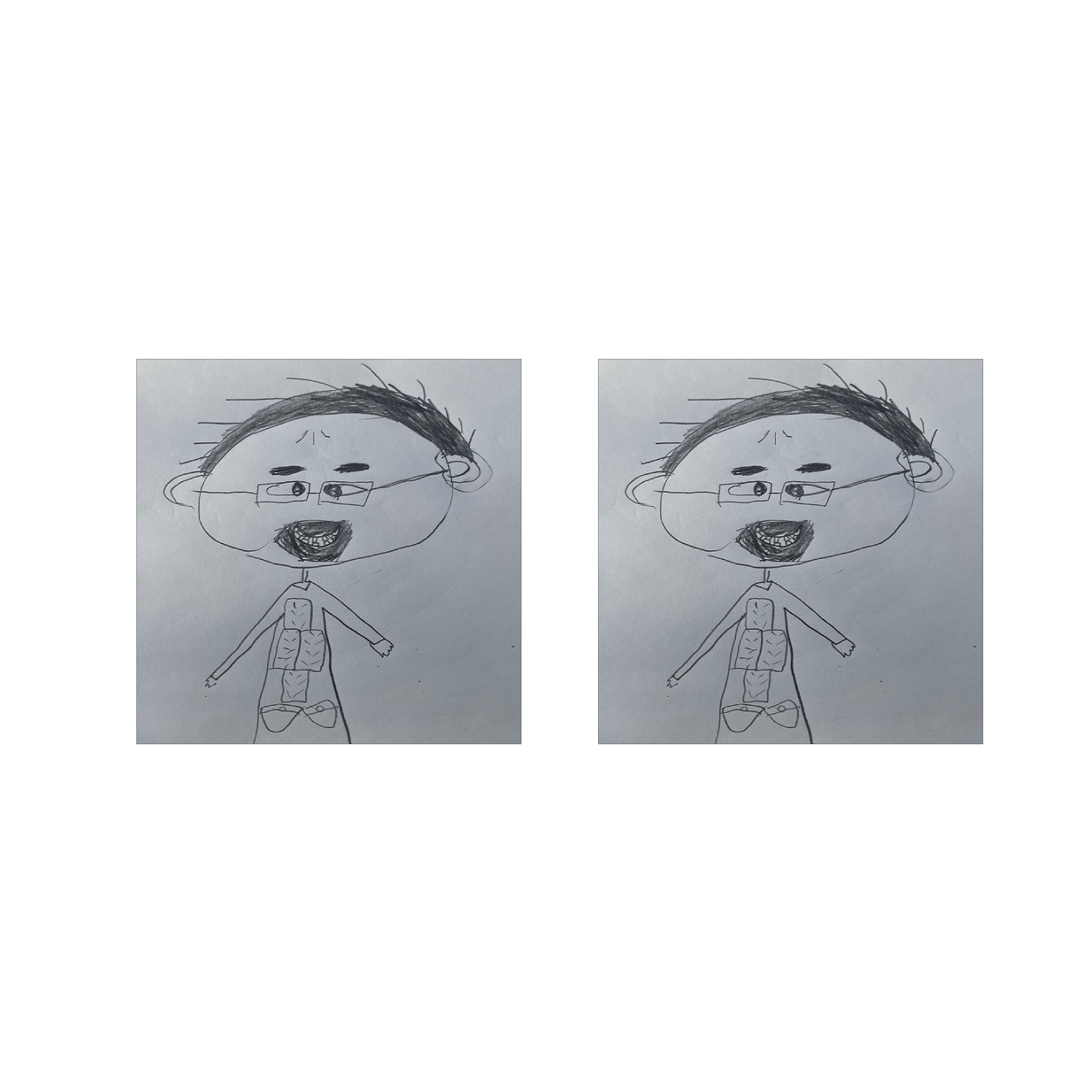
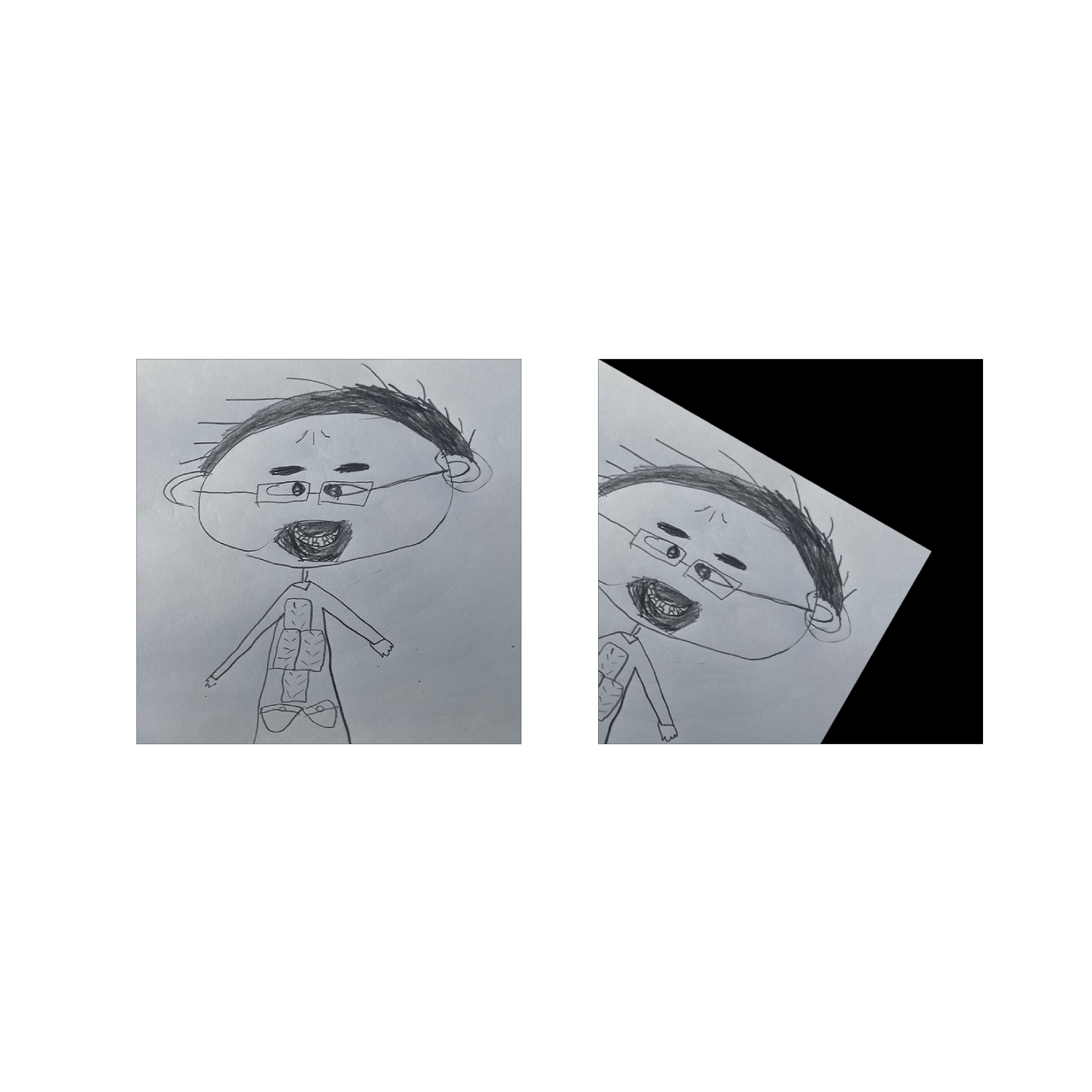
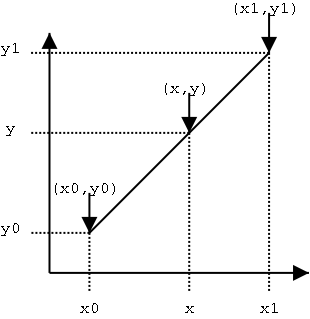
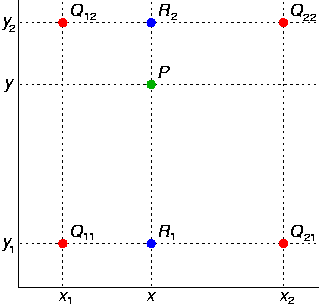

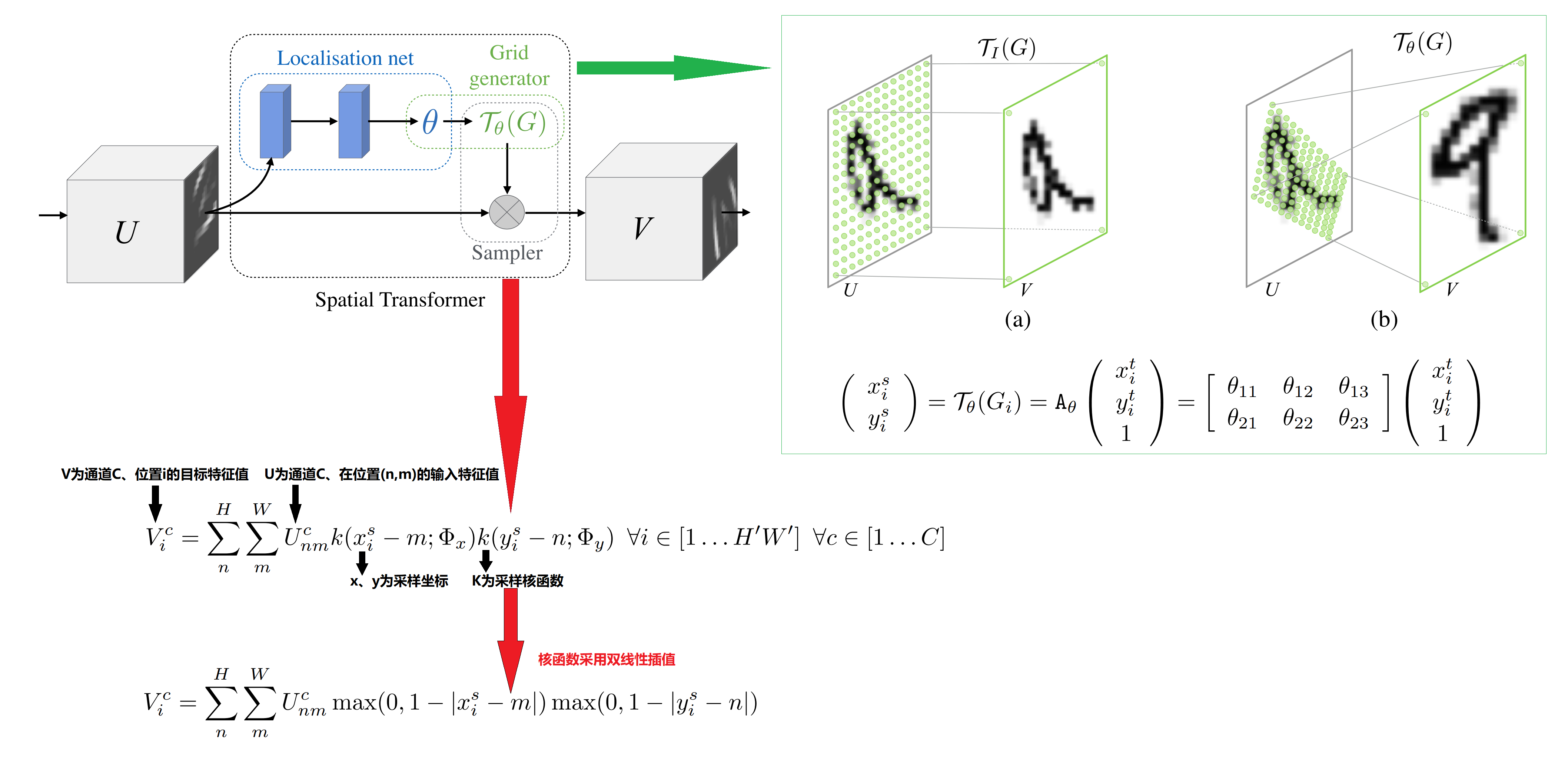
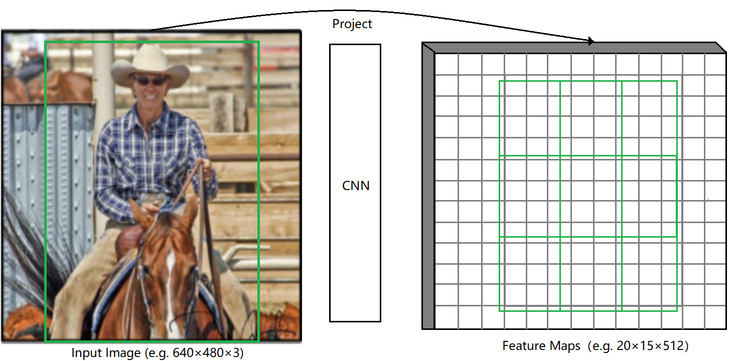
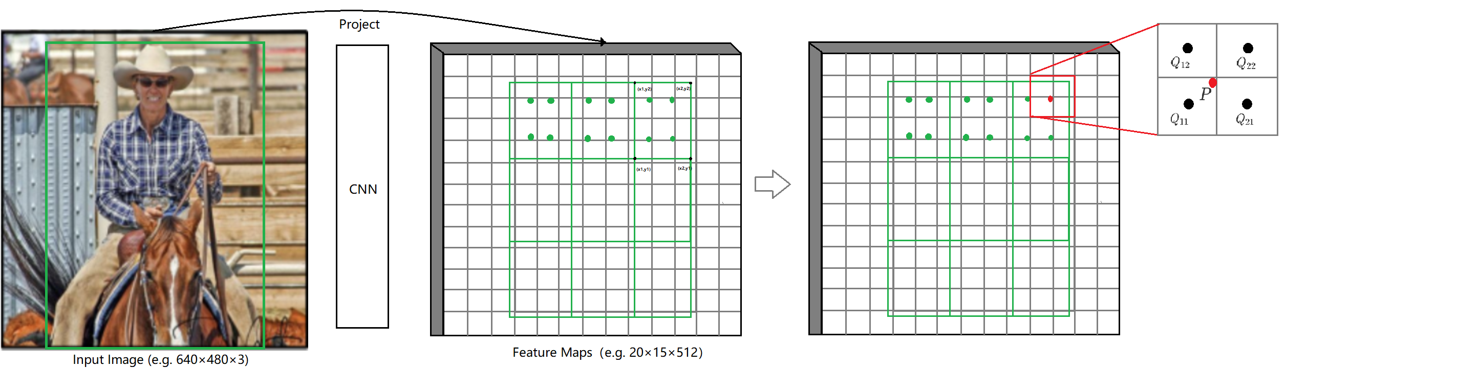
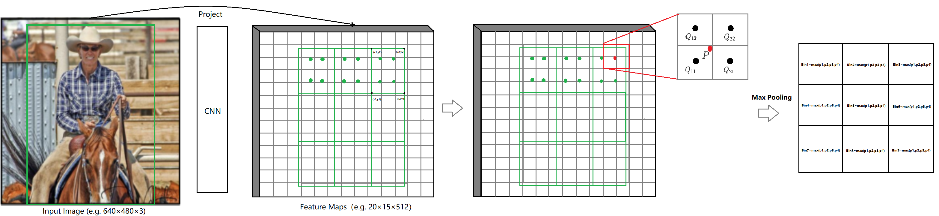
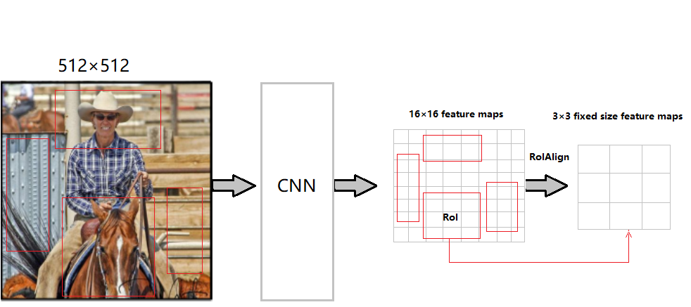
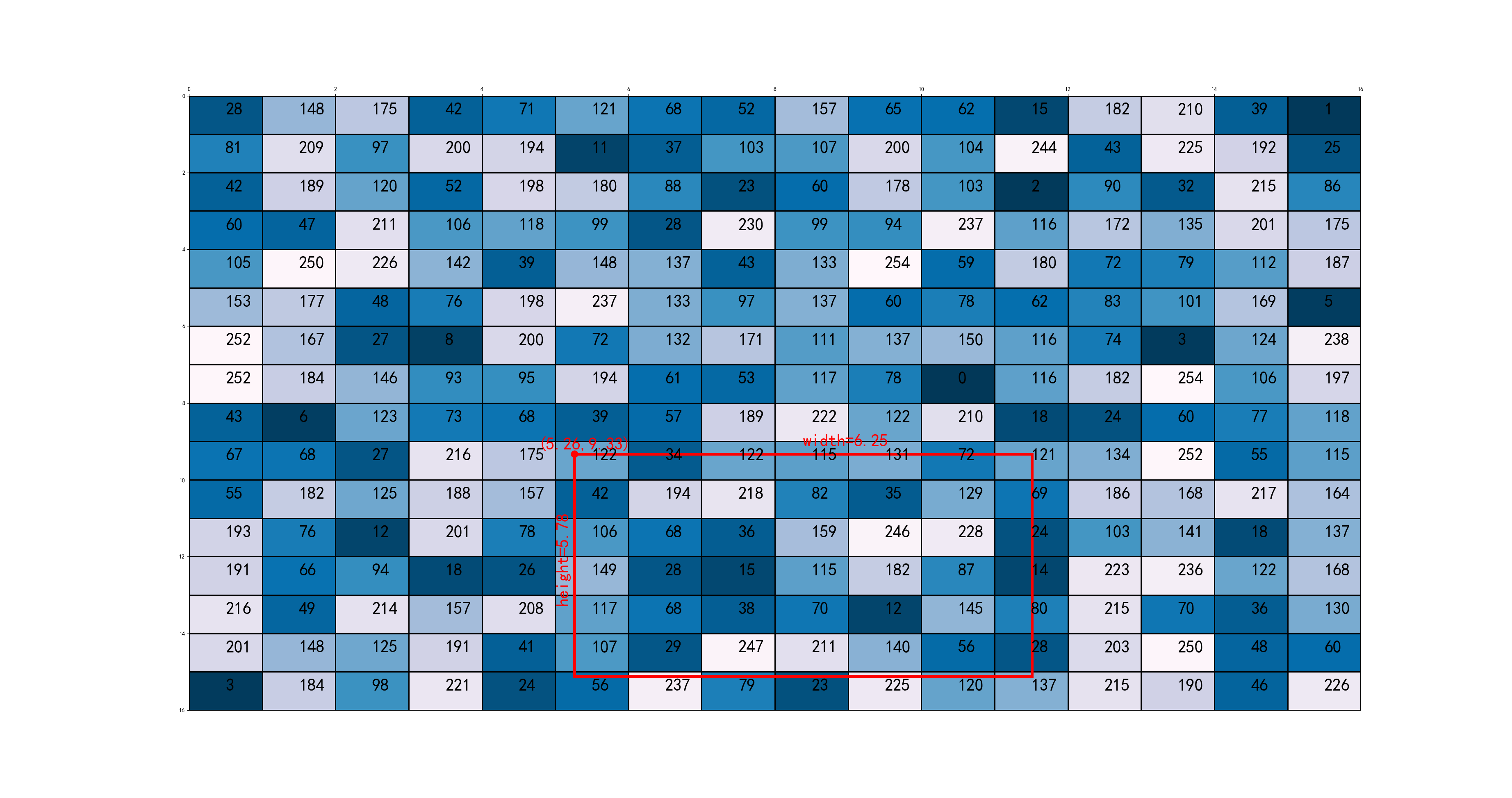


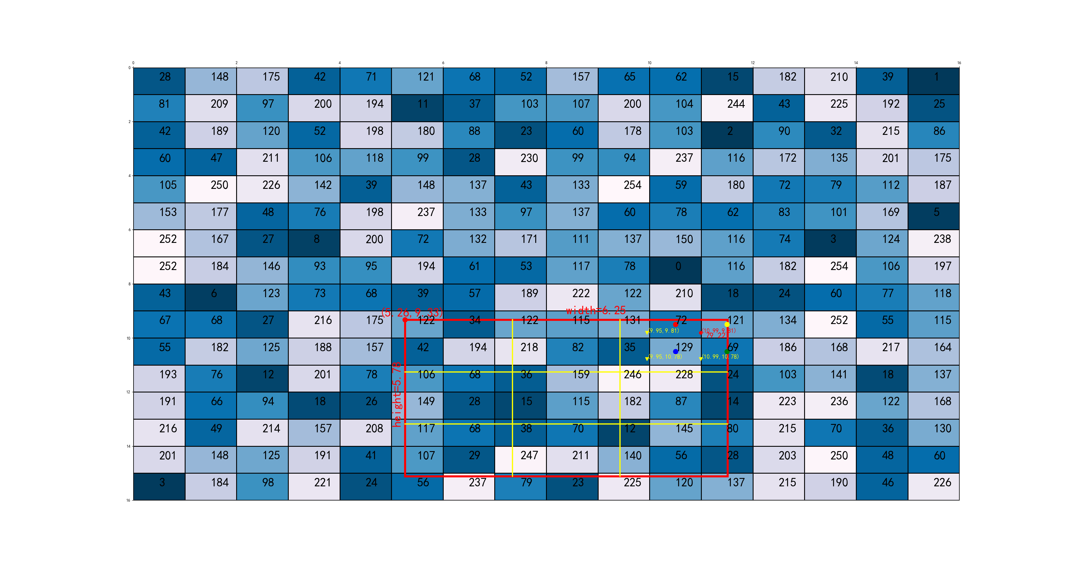
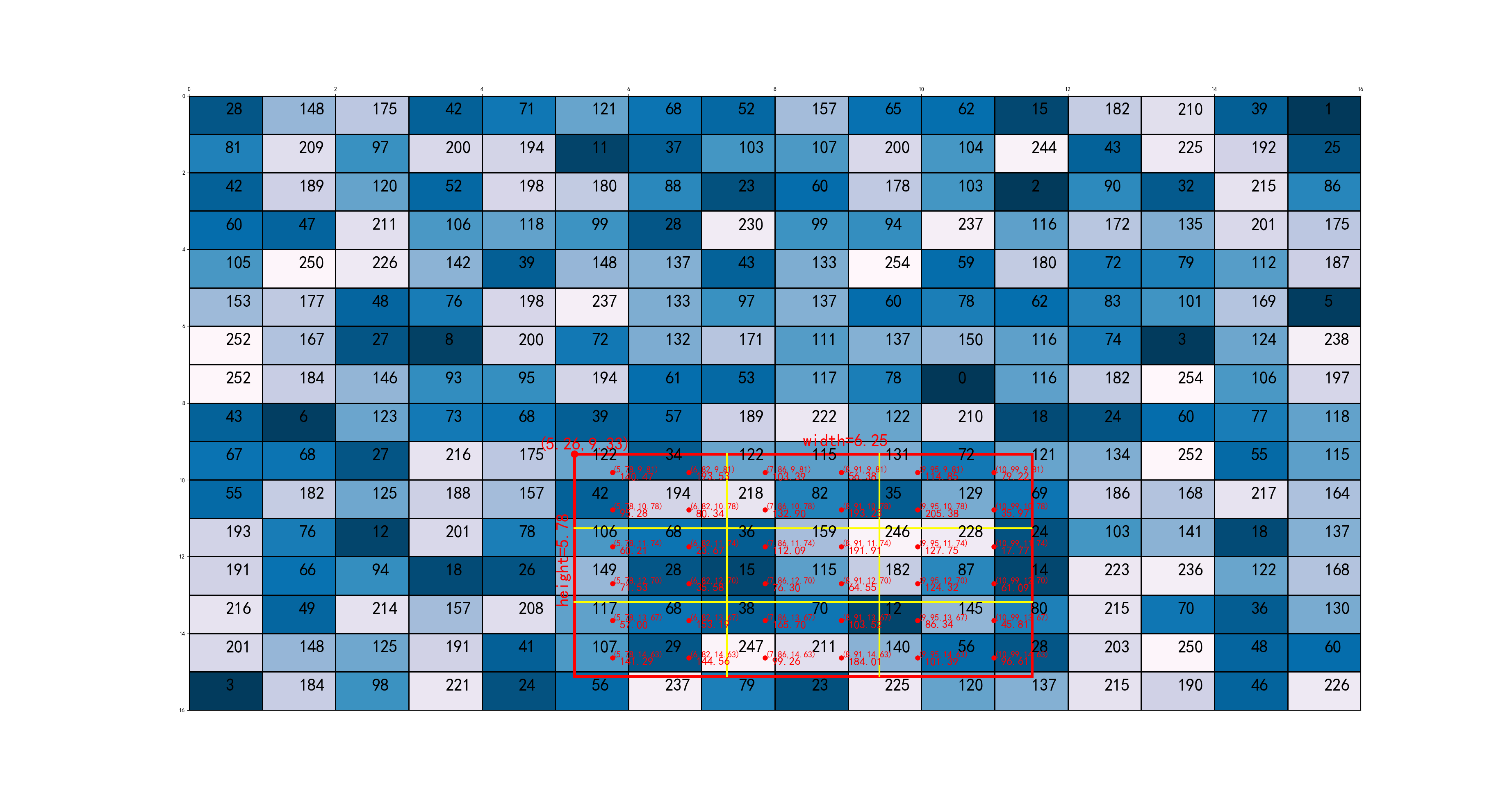
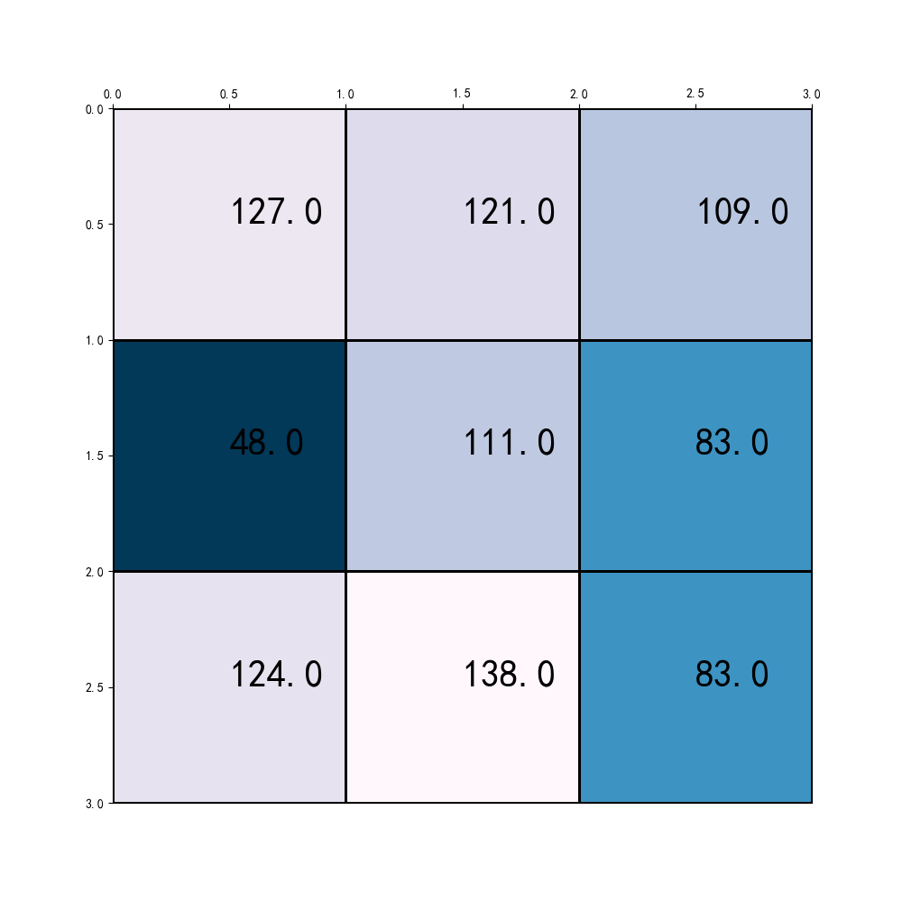
8.9.4 网络结构及目标函数
网络结构
下图左右两图分别为:ResNet骨干网络+Head和FPN骨干网络+Head:
![]()
目标函数
对Faster R-CNN做了些许扩展: \[ L=\underbrace{L_{cls}+L_{box}}_{Faster R-CNN}+\underbrace{L_{mask}}_{MaskR-CNN} \]
Faster R-CNN部分:
\[ \underbrace{L(p,u,t^u,v)}_{\begin {align} p&:预测分类\\u&:分类标注\\t^u&:分类u的预测bbox\\v&:bbox标注 \end{align}}=\underbrace{L_{cls}(p,u)}_{log\text{ }loss}+\underbrace{\lambda[u\geq 1]}_{[u\geq 1]=\left\{\begin{matrix}1 &若 u \geq 1\\0&其他\end{matrix}\right.} \cdot \underbrace{L_{box}(t^u,v)}_{smooth\text{ }L1\text{ }loss} \] 其中: \[ \begin {align} log\text{ }loss&:-logp_u=-ulog (p)-(1-u)log(1-p)\\ smooth\text{ }L1\text{ }loss&:\sum_{i \in \{x,y,w,h\}}smooth_{L_i}(t_i^u-v_i)\\ smooth_{L_i}(x)&=\left\{\begin{matrix}0.5x^2 \quad &若 |x|<1\\|x|-0.5&其他\end{matrix}\right.\end{align} \]
Mask部分: \[ \begin {align} L_{mask}&= - \frac{1}{m×m} \sum_{i=1}^m \sum_{j=1}^m \big[ u_{ij} \log y^k_{ij} + (1-u_{ij}) \log (1- y^k_{ij}) \big]\\ y_{ij}&:位置(i,j)处像素针对分类k的预测mask值\\ u_{ij}&:位置(i,j)处像素的标注mask值\\ m&:mask \text{ } feature \text{ } map矩阵维度(m×m)\\ \end{align} \] 注意,对每个像素都会有一个二分类结果,以及每个类都会有一个mask矩阵(m×m)输出,所以总共会有\(K\cdot(m×m)\)个sigmoid输出,而如果RoI判定为第\(k\)个分类,则损失函数\(L_{mask}\)为第\(k\)个分类下的平均二分类交叉熵损失(average binary cross-entropy loss),也就是说所有分类之间不会产生竞争,文中这部分效果如下:
![]()
分割效果:
![]()
![]()
![]()
![]()
![]()
![]()