机器学习中的自动微分(Automatic Differentiation)

本文对自动微分机器原理做了简单介绍。

机器学习中的自动微分

计算机求解微分可以分成四类方法：

手工求解

在《机器学习与人工智能技术分享-第四章 最优化原理》中介绍了大量手工求解微分的算法，它们大都是通过泰勒展开式推导出的，只利用梯度求优化问题的叫一阶优化算法，如SGD，利用Hessians矩阵求解的是二阶优化算法，如L-BFGS， 这些算法的特点是能够很灵活自主高效的求解优化问题，包括一些目标函数不可微的问题，研究人员需要有很强的数学背景和代码实现能力，缺点是耗时且容易出错，代码调试也比较复杂。

数值微分

原理很简单，就是利用导数的定义求解，所以实现起来也不复杂，形式化描述是： 假设有\(n\)元目标函数\(f(X)=f(x_1,x_2,....x_n):\mathbb{R} \rightarrow \mathbb{R}\)，求解其梯度，可以对它的每个维度分别使用导数定义求解： \[\frac{\partial f(X)}{\partial x_i} \approx \frac{f(X+he_i)-f(X)}{h}\] 其中\(e_i\)是第\(i\)维的单位向量，\(0<h\ll 1\)是一个微小步长，最后得到： \[\nabla f(X)=(\frac{\partial f}{\partial x_1},\frac{\partial f}{\partial x_2},...,\frac{\partial f}{\partial x_n})^T\]

例如，求解\(f(x_1,x_2)=x_1+x_2^2\)，假设取\(h=0.000001\)，则： \[\begin{equation} \frac{\partial f(X)}{\partial x_i}\approx\left\{ \begin{aligned} \frac{f(x_1+0.000001,x_2)-f(x_1,x_2)}{0.000001}&=1 \\ \frac{f(x_1,x_2+0.000001)-f(x_1,x_2)}{0.000001}&=2x_2+0.000001 \end{aligned} \right. \end{equation} \] 如\(f'(1,1)=(1,2.000001)^T\)。

不过由于这种方法的缺点是：

1)、多元函数的每个维度都要算一遍，即\(O(n)\)的时间复杂度，尤其在当今的机器学习问题中，这个维度非常大，会导致这种方法完全无法落地；

2)、由于这种求解方法天然是病态（ill-conditioned）且不稳定的（比如计算机的计算精度本来就是有限的），所以每个维度的每个\(h\)的取值要很小心，否则就会出现较大误差，这种误差一般有两种：截断误差(Truncation error)和舍入误差(Roundoff error)，

截断误差，简单说就是因为截断操作导致的误差，例如：无穷级数: \[S_n=\lim_{n \to \infty} \sum_{1}^n\frac{1}{2^n}=1\] 我们只能在有限的步数内做估计，如取：\(n=6\)，则\(S_6=\frac{63}{64}\)，截断误差为：\(0.015625\)。

舍入误差，简单说就是类似四舍五入这样的操作导致的误差，计算机在表示数字的能力上存在数量级和精度限制，某些数值操作对舍入误差非常敏感，且误差会被累积放大。

为了缓解上面的误差，人们想了很多办法，例如使用center difference估计法，如下： \[\frac{\partial f(X)}{\partial x_i} = \frac{f(X+he_i)-f(X-he_i)}{2h}+O(h^2)\]

以函数\(f(x)=64x(1−x)(1−2x)^2(1−8x+8x^2)^2\)为例，两种方法比较如下：

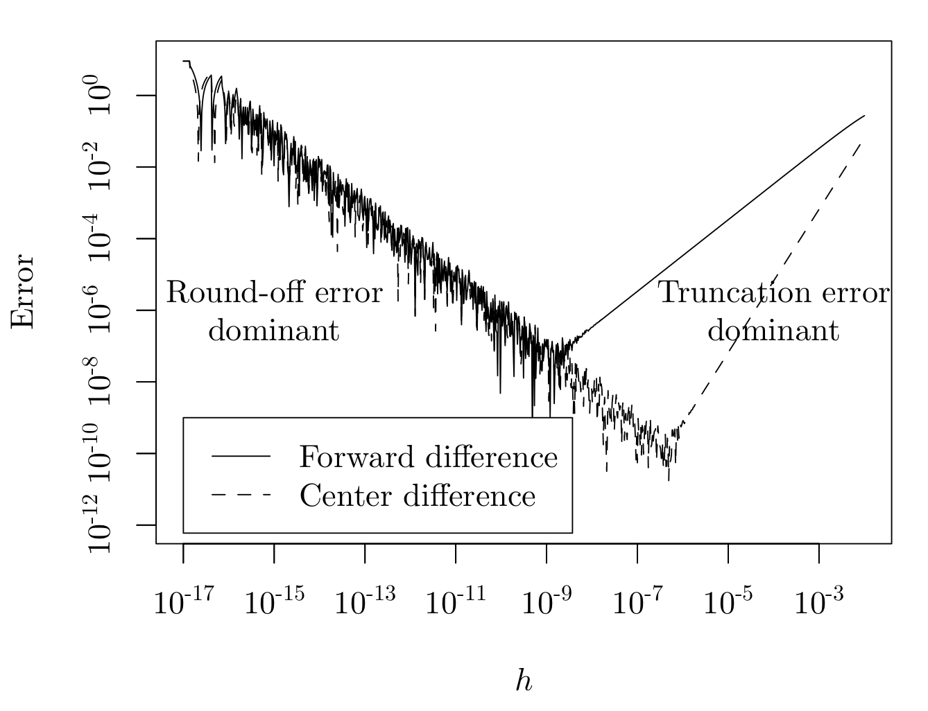
其中： \(E_{forward} (h, x_0 ) =\left|\frac{f(x_0+h)-f(x_0)}{h}-\frac{d}{dx}f(x)|_{x_0}\right|\)， \(E_{center} (h, x_0 )=\left|\frac{f(x_0+h)-f(x_0-h)}{2h}-\frac{d}{dx}f(x)|_{x_0}\right|\)，\(x_0=0.2\) ，对截断误差和舍入误差的tradeoff体现在\(h\)的取值上，即使是改进后的Center difference，稍有不慎误差也会被放大。

符号微分

符号微分，顾名思义就是把微分的基本规则符号化，通过自动操作表达式从而获得各种衍生表达式，例如下面的积分规则： \[\begin{equation} \left\{ \begin{aligned} &\frac{d}{dx}(f(x)+g(x))\rightarrow\frac{d}{dx}f(x)+\frac{d}{dx}g(x) \\ &\frac{d}{dx}(f(x)g(x))\rightarrow g(x)\frac{d}{dx}f(x)+f(x)\frac{d}{dx}g(x) \end{aligned} \right. \end{equation} \]

有了这些规则后，可以把输入变成一个由一系列符号表达式组成的树形结构，以前比较著名的深度学习框架Theano用的就是这种方式，但也正是由于这种比较“机械式”的展开，而没有通过复用和仅存储中间子表达式值的方式来简化计算，导致出现表达式成指数级膨胀。 例如函数：\(h(x) = f (x)g(x)\)，对其应用导数的乘法规则有： \[ \frac{d}{dx}h(x)= g(x)\frac{d}{dx}f(x)+f(x)\frac{d}{dx}g(x) \] 这个式子中，\(g(x)\)与\(\frac{d}{dx}g(x)\)是相互独立各算各的，显然一个不小心，它们的公用部分就无法复用，随便一个例子：\(g(x)=6+e^x\)，\(\frac{d}{dx}g(x)=e^x\)，公共部分重复计算。

如果我们更关心输入函数的导数能否准确被算出，而不是它的符号表达本身的话，是可以通过复用及仅存储中间子表达式值的方式来简化计算的，这种思想也是自动微分的基础之一，如下图的例子，对函数\(l_{n+1} = 4l_n (1 − l_n ), l_1 = x\)做表达式展开：

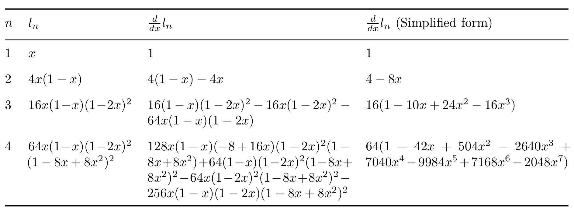
其中第三列是以符号微分形式展开，显然随着式子复杂度上升，展开式复杂度急剧上升，第四列是中间字表达式简化后的形式，复杂度比原始形式大大下降。

自动微分(AD)

通过定义一个有限基本运算的集合，这些基本运算的求导数方法已知，包括一元运算（如：负数、开根号等）、二元运算（如：加、减、乘、除等）、超越函数（如：指数函数、三角函数、反三角函数、对数函数等），利用链式法则结合这些基本运算的导数，通过延迟 计算的方式来计算整个函数的导数，相比符号微分等其他方法，不但能处理封闭表达式（closed-form expressions），还可以支持控制流，如分支、循环、递归和过程调用等，这里解释下什么叫封闭表达式。

封闭表达式(Closed-Form Expressions)

简单说就是能用固定数量操作符表达的式子。

例如：\(y=2+4+6+...+2n\)不是封闭表达式，而\(y=\sum\limits_{i=1}^{n}2i=n(n+1)\)就是封闭表达式。常见的封闭形式举例： \[ \begin{aligned} & \sum\limits_{i=m}^{n}c=(n - m +1)c\\ & \sum\limits_{i=1}^{n}i=\frac{n(n+1)}{2}\\ & \sum\limits_{i=1}^{n}i^2=\frac{n(n+1)(2n+1)}{6}\\ & \sum\limits_{i=0}^{n}a^i=\frac{a^{n+1}-1}{a-1}(a\neq1)\\ & \sum\limits_{i=1}^{n}ia^i=\frac{a-(n+1)a^{n+1}+na^{n+2}}{(a-1)^2}\\ \end{aligned} \]

问题：找到\(2 + 2^2 \cdot 7 + 2^3 \cdot 14 +...+ 2^n (n-1)\cdot 7\)的封闭形式。 解： \[ \begin{aligned} y=& 2 + 2^2 \cdot 7 + 2^3 \cdot 14 +...+ 2^n (n-1)\cdot 7\\ =& 2+\sum\limits_{i=2}^{n}2^i(i-1)\cdot 7\\ =& 2+7\sum\limits_{i=2}^{n}(i-1)2^i\\ =& 2+7\sum\limits_{i=1}^{n-1}i2^{i+1}\\ =& 2+14\sum\limits_{i=1}^{n-1}i2^i\\ =& 2+14(2-n2^n+(n-1)2^{n+1}) \end{aligned} \]

对偶数

数学本质上是由人类通过逻辑抽象思维对事物主观定义出结构和模式并以工具形式存在，用于解决实际问题的。而抽象逻辑是需要自洽的，所以在不同应用范围会产生递进的不同工具：

例如，复数定义为： \[z=a+bi\] 其中\(a\)和\(b\)都是实数且\(i^2=1\)，复数在实际中有广泛的应用。(ps：我最喜欢欧拉公式：\(e^{ix}=\cos x+i\sin x\)，尤其当\(x=\pi\)时，\(e^{i\pi}+1=0\))

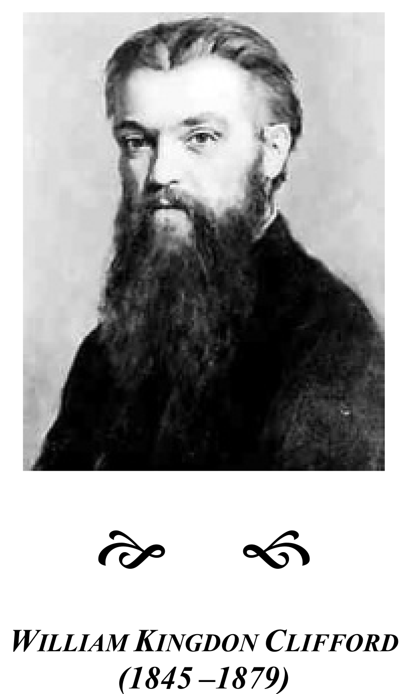
类似复数，在19世纪后期，W. Clifford定义和发展出了对偶数，即： \[z=a+b\epsilon\] 其中\(a\)和\(b\)都是实数且\(\epsilon^2=0\)。

那么对偶数有什么用呢？看到这个定义，我第一个想到的是微分定义中的无穷小量\(dx\)，第二个想到的是，函数的泰勒展开式的2阶及以上的余项部分。 假设\(f:\mathbb{R} \rightarrow \mathbb{R}\)是任意函数，那么在\(x+\epsilon\)处做泰勒展开，如下： \[ f(x+\epsilon)=f(x)+f'(x)\epsilon+ O(\epsilon^2) \] 其中\(O(\epsilon^2) \rightarrow0\)。显然\(f(x)+f'(x)\epsilon\)就是个对偶数，所以有对偶函数： \[ \hat f(\hat x)=f(x)+f'(x)\epsilon \] 简化表示为： \[ \hat f(\hat x)=\{f_0,f_1\},\text{where } f_0=f(x) \text{ and }f_1=f'(x). \] 对复合函数\(f(g(x))\)，根据链式法则有：\((f(g(x)))'=f'(g(x))g'(x)\)有： \[ \hat f(\hat g)=f(g(x))+(f(g(x)))'\epsilon=f(g(x))+f'(g(x))g'(x)\epsilon \] 简写为： \[ \hat f(\hat g)=\{f_0(g_0),f_1(g_0)g_1\} \] 对更复杂的函数\(h(x)=f(g(u(x)))\)有 \[ \hat f(\hat g(\hat u))=\{f_0(g_0(u_0)),f_1(g_0(u_0))g_1(u_0)u_1\} \] 也就是只需要执行一次链式求导就能直接求出\(h'(x)\)（隐含链式求导是延迟执行的），这就是利用对偶数求解某个函数导数的威力，这个就是自动微分前向模式(Forward Mode of AD)的理论依据。

再进一步，定义新的对偶数： \[ \widetilde r=a+b\epsilon_1+c\epsilon_2, \widetilde r=\{a,b,c\} \] 其中\(\{a,b,c\}\in \mathbb{R}\)，\(i,j\in\{1,2\}\)满足关系： \[ \begin{equation} \epsilon_i\cdot \epsilon_j=\left\{ \begin{aligned} &0&\text{ if }i+j>2, \\ &2\epsilon_{i+j}&\text{ otherwise.} \end{aligned} \right. \end{equation} \] 把泰勒展开式展开到二阶： \[ \begin{aligned} f(\widetilde x)=&f(x)+f'(x)\epsilon_1+\frac{1}{2}f''(x)\epsilon_1^2\\ =&f(x)+f'(x)\epsilon_1+f''(x)\epsilon_2 \end{aligned} \] 简写为： \[ \begin{aligned} \widetilde f(\widetilde x)=&\{f(x),f'(x),f''(x)\}\\ =&\{f_0,f_1,f_2\} \end{aligned} \]

以矩阵形式看，定义： \[ \begin{aligned} I=&\left[ \begin{matrix} 1 & 0 & 0 \\ 0 & 1 & 0 \\ 0 & 0 & 1 \end{matrix} \right]\\ \epsilon_1=&\left[ \begin{matrix} 0 & 1 & 0 \\ 0 & 0 & 1 \\ 0 & 0 & 0 \end{matrix} \right]\\ \epsilon_2=&\left[ \begin{matrix} 0 & 0 & 1/2 \\ 0 & 0 & 0 \\ 0 & 0 & 0 \end{matrix} \right]\\ \end{aligned} \] \(X=xI+\epsilon_1\)，则： \[ f(X)=f(x)I+f'(x)\epsilon_1+f''(x)\epsilon_2 \] 同样有： \[ \widetilde f(\widetilde x)=\{f_0,f_1,f_2\},\text{ and }f_0=f(x),f_1=f'(x),f_2=f''(x). \] 对复合函数\(f(g(x))\)就有： \[ \widetilde f(\widetilde g)=\{f_0(g_0),f_1(g_0)g_1,f_2(g_0)g_1^2+f_1(g_0)g_2\}. \] 这个式子最核心的价值除了前面说的只需要执行一次链式求导就能直接求出目标函数的导数（这个导数就是对偶数的第二/对偶部分）外，导数结果不存在截断误差和舍入误差。

常用的对偶数推论有： \[ \begin{aligned} 1.&(a+b \epsilon)+(c+d \epsilon)=a+c+(b+d)\epsilon\\ 2.&(a+b \epsilon)\cdot(c+d \epsilon)=ac+(ad+bc)\epsilon\\ 3.&\frac{a+b \epsilon}{c+d \epsilon}=\frac{a}{c}+\frac{bc-ad}{c^2}\epsilon\\ 4.&-(a+b \epsilon)=-a-b\epsilon\\ 5.&P(a) = p_0 + p_1a + p_2a^2 + · · · + p_na^n \text{ 在}a+b\epsilon\text{处对偶形式为}p(a+b\epsilon)=p(a)+p'(a)b\epsilon\\ 6.&sin(a+b\epsilon )=sin(a)+cos(a)b\epsilon\\ 7.&cos(a+b\epsilon )=cos(a)-sin(a)b\epsilon\\ 8.&e^{a+b\epsilon}=e^a+be^a\epsilon\\ 9.&log(a+b\epsilon)=log(a)+\frac{b}{a}\epsilon \text{ and }a\neq 0\\ 10.&\sqrt{a+b\epsilon}=\sqrt{a}+\frac{b}{2\sqrt{a}}\epsilon \text{ and }a\neq 0\\ 11.&(a+b\epsilon)^n=a^n+na^{n-1}b\epsilon\\ \end{aligned} \]

举个例子：求函数\(f(x)=x-e^{-sin(x)}\)的导数\(f'(x)\)，有： \[ \begin{aligned} f(x+\epsilon)&=x+\epsilon-e^{-sin(x+\epsilon)}\\ &=x+\epsilon-e^{-(sin(x)+cos(x)\epsilon)}\\ &=x-e^{-sin(x)}+(1+cos(x)\cdot e^{-sin(x)})\epsilon \end{aligned} \] 即：\(\widetilde f(\widetilde x)=\{x-e^{-sin(x)},1+cos(x)\cdot e^{-sin(x)}\}\) 所以可以取出对偶部，直接得到\(f'(x)=1+cos(x)\cdot e^{-sin(x)}\)。

前向模式自动微分(Forward mode AD)

前向模式的自动微分等价于执行基于对偶数的函数，举个例子，求函数\(f(x)=x\sin(x^2)\)在点\(x=6\)处的导数：

原始问题	前向模式
\(w_1=x\)	\(\dot{w_1}=1\)
\(w_2=w_1^2\)	\(\dot{w_2}=2w_1\dot{w_1}=2x\)
\(w_3=\sin(w_2)\)	\(\dot{w_3}=\cos(w_2)\dot{w_2}=2x\cos(x^2)\)
\(w_4=w_1w_3\)	\(\dot{w_1}w_3+w_1\dot{w_3}=\sin(x^2)+2x^2\cos(x^2)\)

计算图如下：

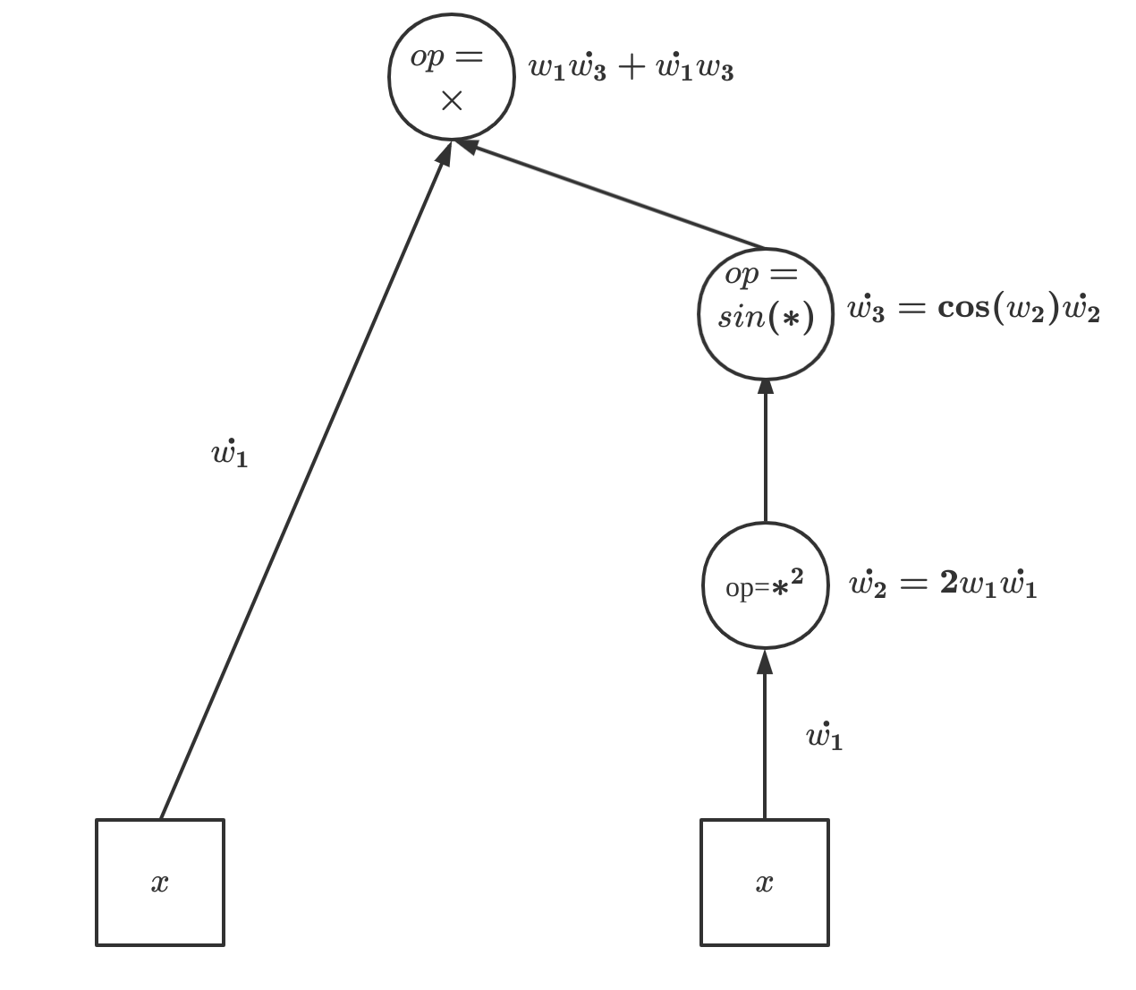
所以在\(x=6\)处原函数的导数为：\(f'(6)=\sin(36)+52\cos(36)=-10.205\)，用对偶数推导如下： \[ \begin{aligned} \text{set}&\\ x&=6+\epsilon \\ u&=x^2\\ &=(6+\epsilon)^2\\ &=36+12\epsilon\\ \text{then}&\\ v&=\sin(u)\\ &=\sin(36+12\epsilon)\\ &=\sin(36)+12\cos(36)\epsilon\\ \text{finally}&\\ w&=x\sin(v)\\ &=(6+\epsilon)(\sin(36)+12\cos(36)\epsilon)\\ &=6\sin(36)+(\sin(36)+72\cos(36))\epsilon \end{aligned} \] 所以利用对偶数同时求得：\(f(6)=6\sin(36)=-5.95\)和\(f'(6)=\sin(36)+72\cos(36)=-10.205\)。

多元函数的例子，计算函数\(f(x,y,z)=xy\cos(xz)\)在点\((-2,3,-6)\)处的梯度向量：

原始问题	前向模式
\(t=xy\)	\(\dot{t}=[y,x,0]\)
\(u=xz\)	\(\dot{u}=[z,0,x]\)
\(v=\cos(u)\)	\(\dot{v}=-\sin(u)\dot{u}=[-\sin(xz)z,0,-\sin(xz)x]\)
\(w=tv\)	\(\dot{w}=\dot{t}v+t\dot{v}=[y\cos(xz)-xyz\sin(xz),x\cos(xz),-x^2y\sin(xz)]\)

计算图如下：

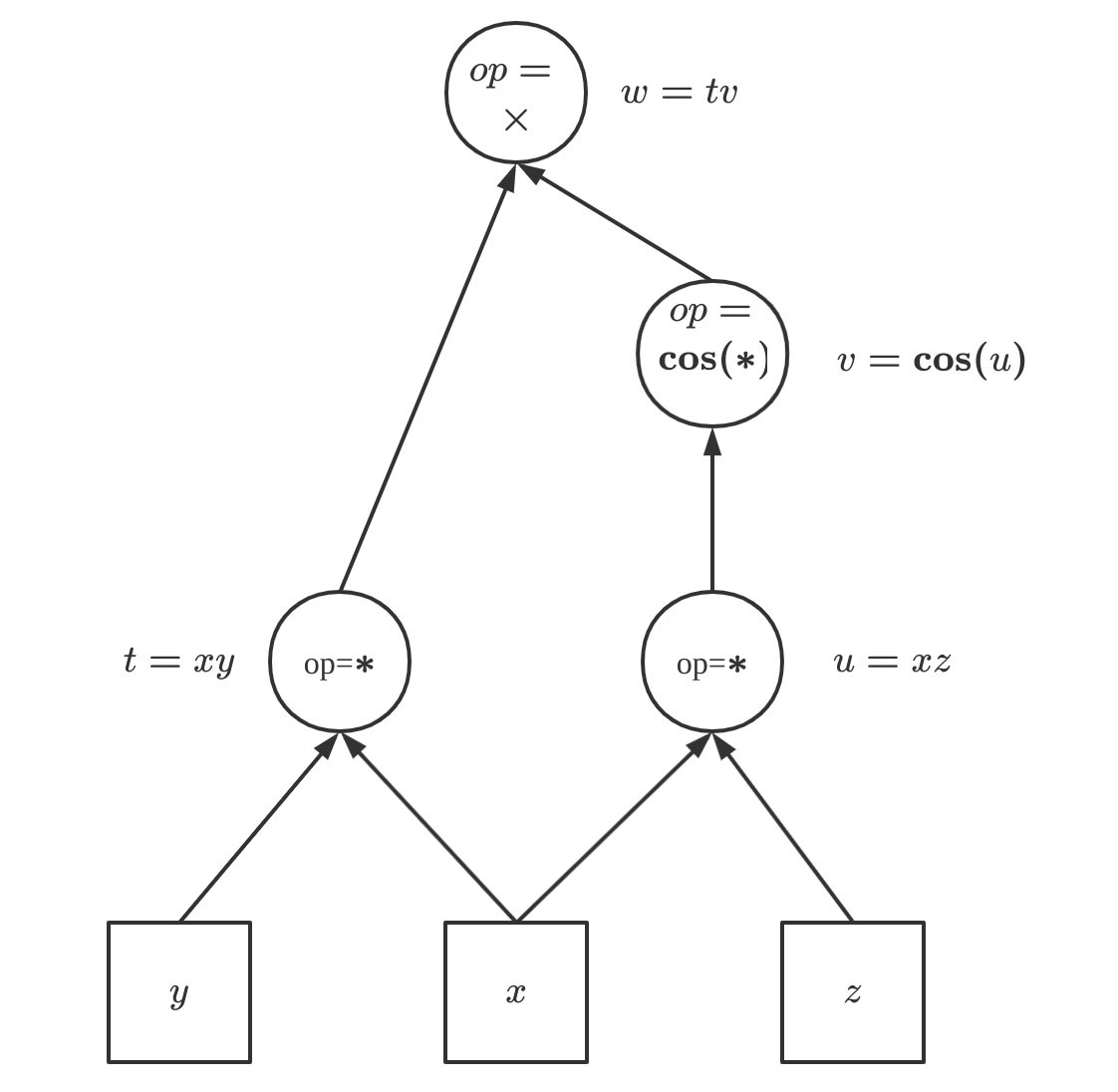
利用对偶数原理和one-hot方式表示，有： \[ \begin{aligned} \text{set}&\\ x&=-2+\epsilon[1,0,0] \\ y&=3+\epsilon[0,1,0]\\ z&=-6+\epsilon[0,0,1]\\ \text{then}&\\ t&=xy\\ &=(-2+\epsilon[1,0,0])(3+\epsilon[0,1,0])\\ &=-6+\epsilon[3,-2,0]\\ u&=xz\\ &=(-2+\epsilon[1,0,0])(-6+\epsilon[0,0,1])\\ &=12+\epsilon[-6,0,-2]\\ v&=\cos(u)\\ &=\cos(12+\epsilon[-6,0,-2])\\ &=\cos(12)-\epsilon\sin(12)[-6,0,-2]\\ w&=tv\\ &=(-6+\epsilon[3,-2,0])(\cos(12)-\epsilon\sin(12)[-6,0,-2])\\ &=-6\cos(12)+\epsilon[-36\sin(12)+3\cos(12),-2\cos(12),-12\sin(12)]\\ &=-5.063+\epsilon[21.848, -1.688, 6.439] \end{aligned} \]

所以利用对偶数同时求得：\(f(-2,3,-6)=-5.063\)和\(\bigtriangledown f(-2,3,-6)=[21.848, -1.688, 6.439]\)。

前向AD代码实践

import math
from deprecated.sphinx import deprecated


class Dual(object):
    """
    封装对偶数及其常用操作符.
    Wraps dual number and its common operators.
    """

    def __init__(self, f0, f1=0.0, var_name='x'):
        """
        初始化对偶数.
        :param f0: 对偶数函数值部分.
        :param f1: 对偶数一阶导数部分.
        """
        self.f0 = f0
        self.f1 = f1
        self.var_name = var_name

    def __add__(self, obj):
        """
        重载对偶数正向加法操作.
        :param obj: 加数.
        :return: 加和结果.
        """
        if isinstance(obj, Dual):
            return Dual(self.f0 + obj.f0, self.f1 + obj.f1)
        elif isinstance(obj, int) or isinstance(obj, float):
            return Dual(self.f0 + obj, self.f1)

        return None

    def __radd__(self, obj):
        """
        重载对偶数反向加法操作.
        :param obj: 被加数.
        :return: 加和结果.
        """
        if isinstance(obj, Dual):
            return Dual(self.f0 + obj.f0, self.f1 + obj.f1)
        elif isinstance(obj, int) or isinstance(obj, float):
            return Dual(self.f0 + obj, self.f1)

        return None

    def __sub__(self, obj):
        """
        重载对偶数正向减法操作.
        :param obj: 减数.
        :return: 减法结果.
        """
        if isinstance(obj, Dual):
            return Dual(self.f0 - obj.f0, self.f1 - obj.f1)
        elif isinstance(obj, int) or isinstance(obj, float):
            return Dual(self.f0 - obj, self.f1)

        return None

    def __rsub__(self, obj):
        """
        重载对偶数反向减法操作.
        :param obj: 被减数.
        :return: 减法结果.
        """
        if isinstance(obj, Dual):
            return Dual(obj.f0 - self.f0, obj.f1 - self.f1)
        elif isinstance(obj, int) or isinstance(obj, float):
            return Dual(obj - self.f0, -self.f1)

        return None

    def __mul__(self, obj):
        """
        重载对偶数正向乘法操作.
        :param obj: 乘数.
        :return: 乘法结果.
        """
        if isinstance(obj, Dual):
            return Dual(self.f0 * obj.f0, self.f0 * obj.f1 + self.f1 * obj.f0)
        elif isinstance(obj, int) or isinstance(obj, float):
            return Dual(self.f0 * obj, self.f1 * obj)

        return None

    def __rmul__(self, obj):
        """
        重载对偶数逆向乘法操作.
        :param obj: 被乘数.
        :return: 乘法结果.
        """
        if isinstance(obj, Dual):
            return Dual(self.f0 * obj.f0, self.f0 * obj.f1 + self.f1 * obj.f0)
        elif isinstance(obj, int) or isinstance(obj, float):
            return Dual(self.f0 * obj, self.f1 * obj)

        return None

    def __truediv__(self, obj):
        """
        重载对偶数正向除法操作.
        :param obj: 除数.
        :return: 除法结果.
        """
        if isinstance(obj, Dual) and obj.f0 != 0:
            return Dual(self.f0 / obj.f0, (self.f1 * obj.f0 - self.f0 * obj.f1) / obj.f0 ** 2)
        elif isinstance(obj, int) or isinstance(obj, float) and obj != 0:
            return Dual(self.f0 / obj, self.f1 / obj)

        return None

    def __rtruediv__(self, obj):
        """
        重载对偶数反向除法操作，obj若为整数或浮点数会被自动转为对偶数.
        :param obj: 被除数.
        :return: 除法结果.
        """
        if isinstance(obj, Dual) and self.f0 != 0:
            return Dual(obj.f0 / self.f0, (obj.f1 * self.f0 - obj.f0 * self.f1) / self.f0 ** 2)
        elif isinstance(obj, int) or isinstance(obj, float) and self.f0 != 0:
            obj = Dual(obj)
            return Dual(obj.f0 / self.f0, (obj.f1 * self.f0 - obj.f0 * self.f1) / self.f0 ** 2)

        return None

    def __neg__(self):
        """
        重载对偶数取负数操作.
        :return: 取负结果.
        """
        return Dual(-self.f0, -self.f1)

    def __pow__(self, n):
        """
        重载对偶数幂函数操作，要求n必须为整数.
        :param n: 幂.
        :return: 幂函数结果.
        """
        if isinstance(n, int):
            return Dual(self.f0 ** n, n * self.f0 ** (n - 1) * self.f1)

        return None

    def __str__(self):
        """
        重载对偶数字符串函数.
        :return: 对偶数的格式化字符串.
        """
        if self.f1 > 0:
            return '{} = {} + {} ε'.format(self.var_name, self.f0, self.f1)
        else:
            return '{} = {} - {} ε'.format(self.var_name, self.f0, math.fabs(self.f1))

    def print_dual(self):
        """
        格式化打印对偶数.
        :return: 控制台输出.
        """
        print(self)

    @staticmethod
    def sin(x):
        """
        对偶数sine函数.
        :param x: 输入变量.
        :return: 对偶数形式的函数结果.
        """
        if type(x) is Dual:
            return Dual(math.sin(x.f0), math.cos(x.f0) * x.f1)
        elif isinstance(x, int) or isinstance(x, float):
            return Dual(math.sin(x))

    @staticmethod
    def cos(x):
        """
        对偶数cosine函数.
        :param x: 输入变量.
        :return: 对偶数形式的函数结果.
        """
        if type(x) is Dual:
            return Dual(math.cos(x.f0), -math.sin(x.f0) * x.f1)
        elif isinstance(x, int) or isinstance(x, float):
            return Dual(math.cos(x))

    @staticmethod
    def exp(x):
        """
        对偶数e^x函数.
        :param x: 输入变量.
        :return: 对偶数形式的函数结果.
        """
        if type(x) is Dual:
            return Dual(math.exp(x.f0), math.exp(x.f0) * x.f1)
        elif isinstance(x, int) or isinstance(x, float):
            return Dual(math.exp(x))

    @staticmethod
    def log(x):
        """
        对偶数log函数.
        :param x: 输入变量.
        :return: 对偶数形式的函数结果.
        """
        if type(x) is Dual and x.f0 != 0:
            return Dual(math.log(x.f0), x.f1 / x.f0)
        elif isinstance(x, int) or isinstance(x, float):
            return Dual(math.log(x))

    @staticmethod
    def sqrt(x):
        """
        对偶数开根号函数.
        :param x: 输入变量.
        :return: 对偶数形式的函数结果.
        """
        if type(x) is Dual:
            return Dual(math.sqrt(x.f0), x.f1 / (2 * math.sqrt(x.f0)))
        elif isinstance(x, int) or isinstance(x, float):
            return Dual(math.sqrt(x))

    @staticmethod
    @deprecated(version='1.0', reason="This function will be removed soon.")
    def derive(func, f1=1, *args):
        """
        求函数一阶导数.
        :param func: 待求解函数.
        :param f1: 函数一阶导数初始化.
        :param args: 函数参数.
        :return: 一阶导数结果.
        """
        paras = []
        for para in args:
            if not isinstance(para, Dual):
                paras.append(Dual(para, f1))
            else:
                paras.append(para)

        if len(paras) == 1:
            return func(paras[0]).f1
        elif len(paras) == 2:
            return func(paras[0], paras[1]).f1
        else:
            return None

    @staticmethod
    def gradient(func, *args):
        """
        求解指定多元函数的梯度，依据从左到右的变量顺序给出梯度值，
        例如：函数 f(x,y)的梯度为：▽f(x,y)=[f'(x),f'(y)].
        :param func: 待求解函数.
        :param args: 函数输入参数.
        :return: 梯度向量.
        """
        gs = []
        for i in range(len(args)):
            paras = []
            for j in range(len(args)):
                if not isinstance(args[j], Dual):
                    if i == j:
                        paras.append(Dual(args[j], 1))
                    else:
                        paras.append(Dual(args[j], 0))
                else:
                    if i == j:
                        paras.append(Dual(args[j].f0, 1))
                    else:
                        paras.append(Dual(args[j].f0, 0))

            gs.append(func(paras).f1)

        return gs

    @staticmethod
    def newton_raphson(func, x0, u0, n):
        """
        二元函数牛顿-拉森夫法.
        :param func: 待求解函数.
        :param x0: 输入变量1.
        :param u0: 输入变量2.
        :param n: 算法迭代次数.
        :return: 对偶数结果.
        """
        x0d = Dual(x0, 1)
        u0d = Dual(u0)

        for k in range(n):
            fx = func(u0d, x0d)
            fu = Dual.gradient(func, Dual(u0d.f0, 1), x0d)
            u0d = u0d - fx / fu[0]

            print('k={}, {}'.format(k, u0d))

        return u0d


# ----------------------------------


def excf1(*args):
    """
    复合函数示例：f(u(x),x) = cos(u(x)x)−u(x)^3+x+ sin(u(x)^2x)
    :param args: 输入参数(u(x),x).
    :return: 对偶数结果.
    """
    if len(args) == 1 and len(args[0]) == 2:
        u = args[0][0]
        x = args[0][1]
    else:
        u = args[0]
        x = args[1]

    return Dual.cos(u * x) - u ** 3 + x + Dual.sin(u ** 2 * x)


def excf2(*args):
    """
    示例函数：f(u(x),x) = sin(u(x))+x
    :param args: 输入参数(u(x),x).
    :return: 对偶数结果.
    """
    if len(args) == 1 and len(args[0]) == 2:
        u = args[0][0]
        x = args[0][1]
    else:
        u = args[0]
        x = args[1]

    return Dual.sin(u) + x


# ----------------------------------

def exf0(*args):
    """
    示例函数：f(x) = 6x^3 + 2x^2.
    :param args: 输入参数x.
    :return: 对偶数结果.
    """
    if len(args) == 1 and not isinstance(args[0], list):
        x = args[0]
    else:
        x = args[0][0]

    return 6 * x ** 3 + 2 * x ** 2


def dexf0(x):
    """
    一元函数示例：f(x) = 6x^3 + 2x^2的梯度值.
    :param x: 输入参数(x).
    :return: 对偶数结果.
    """
    return Dual.gradient(exf0, x)


def exf1(*args):
    """
    二元函数示例：f(x) = 3x+10y的梯度向量.
    :param x: 输入参数(x,y).
    :return: 对偶数结果.
    """
    x = args[0][0]
    y = args[0][1]
    return 3 * x + 10 * y


def exf2(*args):
    """
    三元函数示例：f(x,y,z)=xysin(yz)的梯度向量.
    :param args: 输入参数(x,y,z)
    :return: 对偶数结果.
    """
    x = args[0][0]
    y = args[0][1]
    z = args[0][2]
    return x * y * Dual.sin(y * z)


def exf3(*args):
    """
    二元函数示例：f(x1,x2)=log(x1)+x1*x2-sin(x2)的梯度向量.
    :param args: 输入参数(x,y,z)
    :return: 对偶数结果.
    """
    x1 = args[0][0]
    x2 = args[0][1]
    return Dual.log(x1) + x1 * x2 - Dual.sin(x2)


def exfox(*args):
    """
    二元函数示例：f(x1,x2)=log(x1)+x1*x2-sin(x2)的梯度向量.
    :param args: 输入参数(x,y,z)
    :return: 对偶数结果.
    """
    x1 = args[0][0]
    x2 = args[0][1]
    return x1 * x2 + Dual.sin(x1)


def exfams(*args):
    """
    二元函数示例：f(x1,x2)=log(x1)+x1*x2-sin(x2)的梯度向量.
    :param args: 输入参数(x,y,z)
    :return: 对偶数结果.
    """
    if len(args) == 1 and not isinstance(args[0], list):
        x = args[0]
    else:
        x = args[0][0]
    return x * Dual.sin(x ** 2)


def exf5(*args):
    """
    三元函数示例：f(x,y,z)=xycos(xz)的梯度向量.
    :param args: 输入参数(x,y,z)
    :return: 对偶数结果.
    """
    x = args[0][0]
    y = args[0][1]
    z = args[0][2]
    return x * y * Dual.cos(x * z)


if __name__ == '__main__':
    x0 = 0.7
    u0 = 1.6
    n = 10

    u = Dual.newton_raphson(excf1, x0, u0, n)
    u.print_dual()
    print("\033[31mf(u(x),x) = cos(u(x)x)−u(x)^3+x+ sin(u(x)^2x) use the newton-raphson algorithm to find u(x) at the "
          "initial value (x0,u0)=({}, {}): \033[0m".format(x0, u0))
    print("\033[31mu(x0)={} and u'(x0)={}\033[0m".format(u.f0, u.f1))
    print("\033[32mf(u(x),x) = sin(u(x))+x at the "
          "initial value (x0,u0)=({}, {}): \033[0m".format(x0, u0))
    g = excf2(u, x0) + Dual(0, Dual.gradient(excf2, u, x0)[1])
    print("\033[32mg(x0)={} and g'(x0)={}\033[0m".format(g.f0, g.f1))

    print("\033[33mf(x) = 6x^3 + 2x^2: f(1) = {} then f'(1) = {}\033[0m".format(exf0(1), dexf0(1)))

    print("\033[31mf(x,y) =3x + 10y gradient vector at point({},{}):{}\033[0m".format(1, 1, Dual.gradient(exf1, 1, 1)))

    print("\033[32mf(x,y,z) =xysin(yz) gradient vector at point({},{},{}):{}\033[0m".format(3, -1, 2,
                                                                                            Dual.gradient(exf2, 3, -1,
                                                                                                          2)))

    print("\033[32mf(x,y,z) =xycos(xz) gradient vector at point({},{},{}):{}\033[0m".format(-2, 3, -6,
                                                                                             Dual.gradient(exf5, -2, 3,
                                                                                                           -6)))

    print("\033[33mf(x1,x2)=log(x1)+x1*x2-sin(x2) gradient vector at point({},{}):{}\033[0m".format(2, 5,
                                                                                                    Dual.gradient(exf3,
                                                                                                                  2,
                                                                                                                  5)))

    print("\033[33mf(x1,x2)=x1*x2+sin(x1) gradient vector at point({},{}):{}\033[0m".format(2, 5,
                                                                                            Dual.gradient(exfox,
                                                                                                          2,
                                                                                                          5)))

    print("\033[33mf(x)=xsin(x**2) gradient vector at point({}):{}\033[0m".format(6,
                                                                                  Dual.gradient(exfams,
                                                                                                6)))

k=0, x = 1.3745071326929446 - 0.11382505528565992 ε
k=1, x = 1.3128464318221855 + 0.058350216540021926 ε
k=2, x = 1.3085520610889037 + 0.11245296805019295 ε
k=3, x = 1.3085322280402245 + 0.11635228047793793 ε
k=4, x = 1.3085322276188782 + 0.11637033108795897 ε
k=5, x = 1.3085322276188782 + 0.11637033147144211 ε
k=6, x = 1.3085322276188782 + 0.11637033147144209 ε
k=7, x = 1.3085322276188782 + 0.11637033147144213 ε
k=8, x = 1.3085322276188782 + 0.1163703314714421 ε
k=9, x = 1.3085322276188782 + 0.1163703314714421 ε
x = 1.3085322276188782 + 0.1163703314714421 ε
f(u(x),x) = cos(u(x)x)−u(x)^3+x+ sin(u(x)^2x) use the newton-raphson algorithm to find u(x) at the initial value (x0,u0)=(0.7, 1.6):
u(x0)=1.3085322276188782 and u'(x0)=0.1163703314714421
f(u(x),x) = sin(u(x))+x at the initial value (x0,u0)=(0.7, 1.6):
g(x0)=1.6658054458395304 and g'(x0)=1.0301710907484147
f(x) = 6x^3 + 2x^2: f(1) = 8 then f'(1) = [22]
f(x,y) =3x + 10y gradient vector at point(1,1):[3, 10]
f(x,y,z) =xysin(yz) gradient vector at point(3,-1,2):[0.9092974268256817, -0.23101126119419035, -1.2484405096414273]
f(x,y,z) =xycos(xz) gradient vector at point(-2,3,-6):[21.848186924213135, -1.6877079174649843, 6.43887501600522]
f(x1,x2)=log(x1)+x1*x2-sin(x2) gradient vector at point(2,5):[5.5, 1.7163378145367738]
f(x1,x2)=x1*x2+sin(x1) gradient vector at point(2,5):[4.583853163452858, 2.0]
f(x)=xsin(x**2) gradient vector at point(6):[-10.205164506616253]

反向模式自动微分(Reverse mode AD)

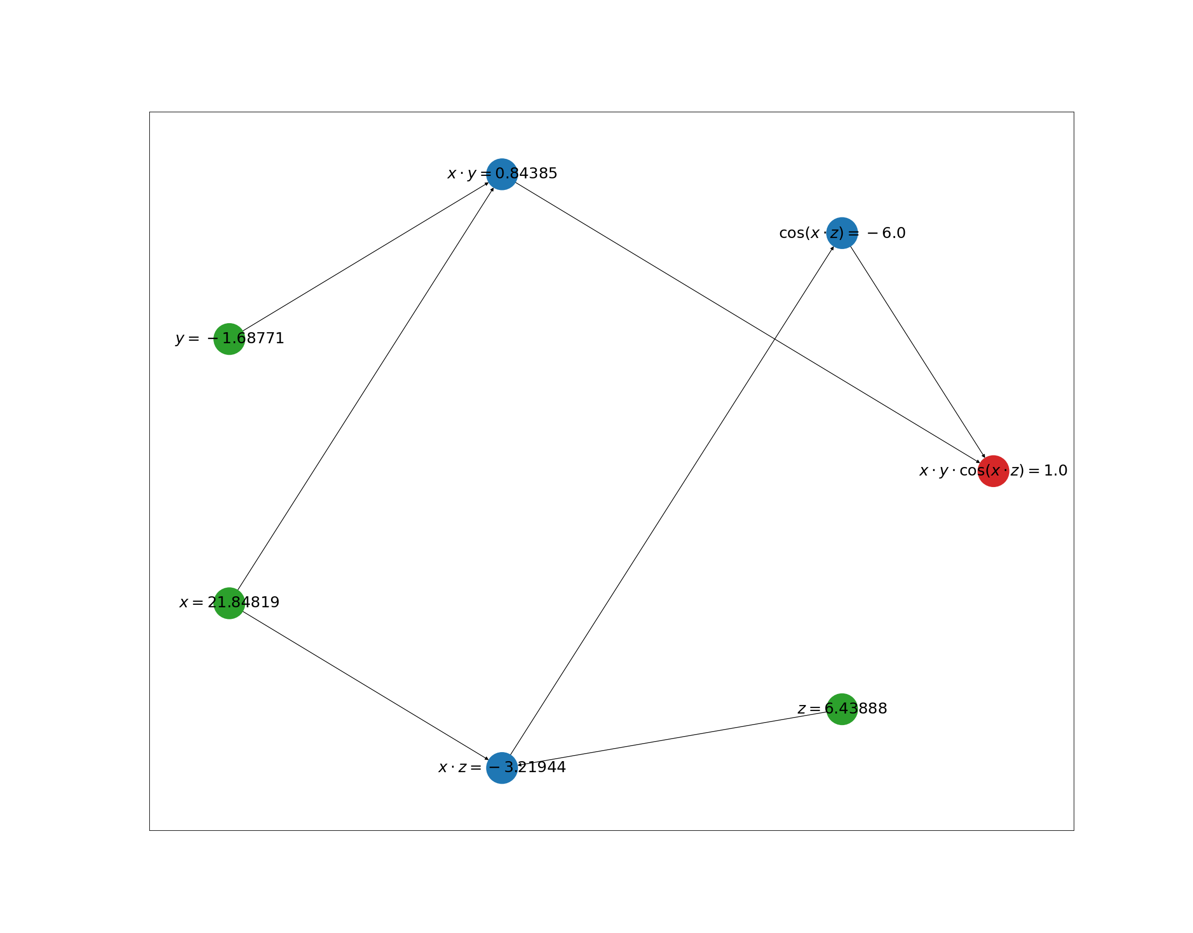
反向模式的自动微分等价于广义上的反向传播算法(BP)，都是从输出反向传播梯度，并用 伴随变量 \(\overline{v}_i=\frac{\partial{y_j}}{\partial v_i}\)补全中间变量， 即，反向AD计算分两个阶段，第一个阶段执行前向AD以计算中间变量导数并记录计算图中的依赖关系，第二个阶段通过将伴随变量反向传播回输入来计算所有导数。 如下图：

依然以函数\(f(x,y,z)=xy\cos(xz)\)在点\((-2,3,-6)\)为例，计算每个中间变量：

原始问题	反向模式
\(x=-2\)	\(\overline{x}=\overline{t}\cdot\frac{\partial t}{\partial x}+\overline{u}\cdot\frac{\partial{u}}{\partial{x}}=vy-tz\sin(u)\)
\(y=3\)	\(\overline{y}=\overline{t}\cdot\frac{\partial t}{\partial y}=vx\)
\(z=-6\)	\(\overline{z}=\overline{u}\cdot\frac{\partial u}{\partial z}=-tx\sin(u)\)
\(t=xy\)	\(\overline{t}=\overline{w}\cdot\frac{\partial w}{\partial t}=v\)
\(u=xz\)	\(\overline{u}=\overline{v}\cdot\frac{\partial v}{\partial u}=-t\sin(u)\)
\(v=\cos(u)\)	\(\overline{v}=\overline{w}\cdot\frac{\partial w}{\partial v}=t\)
\(w=tv\)	\(\overline{w}=\frac{\partial {w}}{\partial {w}}=1\)

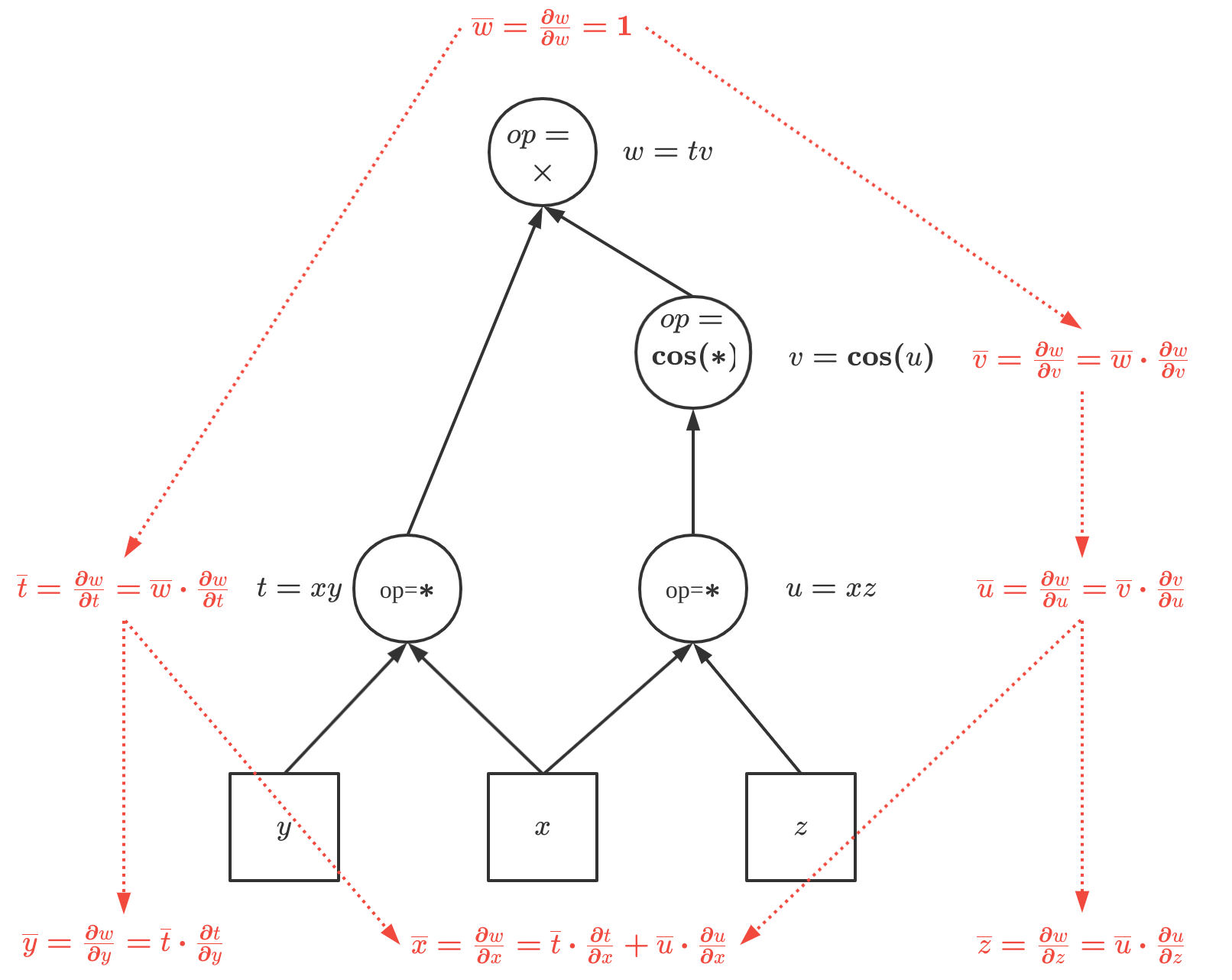
计算图如下：

中间变量和伴随变量计算如下：

\[ \begin{aligned} \overline{w}&=\frac{\partial {w}}{\partial {w}}=1\\ \overline{v}&=\overline{w}\cdot\frac{\partial w}{\partial v}=t=xy=-6\\ \overline{u}&=\overline{v}\cdot\frac{\partial v}{\partial u}=-t\sin(u)=-xy\sin(xz)=-3.219\\ \overline{t}&=\overline{w}\cdot\frac{\partial w}{\partial t}=v=0.8439\\ \overline{z}&=\overline{u}\cdot\frac{\partial u}{\partial z}=-tx\sin(u)=6.4389\\ \overline{y}&=\overline{t}\cdot\frac{\partial t}{\partial y}=vx=-1.6877\\ \overline{x}&=\overline{t}\cdot\frac{\partial t}{\partial x}+\overline{u}\cdot\frac{\partial{u}}{\partial{x}}=vy-tz\sin(u)=21.8482 \end{aligned} \]

计算机求解以上问题有很多方法，其中一种是利用线性代数求解，如下：

把上面的中间变量和伴随变量重新整理下，定义变量：\(x=[\overline{x},\overline{y},\overline{z},\overline{t},\overline{u},\overline{v},\overline{w}]^T\)： \[ \begin{aligned} \overline{x}-3\overline{t}+6\overline{u}=0\\ \overline{y}+2\overline{t}=0\\ \overline{z}+2\overline{u}=0\\ \overline{t}-\overline{w}v=0\\ \overline{u}+\overline{v}\sin(u)=0\\ \overline{v}-\overline{w}t=0\\ \overline{w}=1 \end{aligned} \] 令： \[ \begin{aligned} A&= \left[ \begin{matrix} 1 & 0 & 0 & -3 & 6 & 0 & 0 \\ 0 & 1 & 0 & 2 & 0 & 0 & 0 \\ 0 & 0 & 1 & 0 & 2 & 0 & 0 \\ 0 & 0 & 0 & 1 & 0 & 0 & -v \\ 0 & 0 & 0 & 0 & 1 & \sin(u) & 0 \\ 0 & 0 & 0 & 0 & 0 & 1 & -t \\ 0 & 0 & 0 & 0 & 0 & 0 & 1 \\ \end{matrix} \right]\\ \\ &= \left[ \begin{matrix} 1 & 0 & 0 & -3 & 6 & 0 & 0 \\ 0 & 1 & 0 & 2 & 0 & 0 & 0 \\ 0 & 0 & 1 & 0 & 2 & 0 & 0 \\ 0 & 0 & 0 & 1 & 0 & 0 & -0.8439 \\ 0 & 0 & 0 & 0 & 1 & -0.5366 & 0 \\ 0 & 0 & 0 & 0 & 0 & 1 & 6 \\ 0 & 0 & 0 & 0 & 0 & 0 & 1 \\ \end{matrix} \right]\\ \\ b&=[0,0,0,0,0,0,1]^T \end{aligned} \] 有： \[ Ax=b \] 显然\(A\)是一个稀疏的上三角矩阵，且对角线所有元素\(a_{ij}\neq 0\)，根据Back Substitution回代定理可知，以上式子有唯一解。

反向AD代码实践

1、Back Substitution求解反向AD

import math

import numpy as np


def back_substitution(A, b):
    n = b.shape[0]
    x = np.zeros_like(b)
    for k in range(n - 1, -1, -1):
        x[k] = (b[k] - np.dot(A[k, k + 1:n], x[k + 1:n])) / A[k, k]

    return x


if __name__ == '__main__':
    A = np.array([[1, 0, 0, -3, 6, 0, 0],
                  [0, 1, 0, 2, 0, 0, 0],
                  [0, 0, 1, 0, 2, 0, 0],
                  [0, 0, 0, 1, 0, 0, -math.cos(12)],
                  [0, 0, 0, 0, 1, math.sin(12), 0],
                  [0, 0, 0, 0, 0, 1, 6],
                  [0, 0, 0, 0, 0, 0, 1]])
    b = np.array([0.0, 0, 0, 0, 0, 0, 1])
    x = back_substitution(A, b)
    print(x)

[21.84818692 -1.68770792  6.43887502  0.84385396 -3.21943751 -6.
  1.        ]

2、计算图求解反向AD

还有一种方式是类似tensorflow计算图的方式求反向AD，以下为代码实践：

from abc import ABC
import math

import networkx as nx
import matplotlib.pyplot as plt


class ComputeGraphNode(object):
    """
    定义计算图节点
    """

    def __init__(self, value=0.0, tag=''):
        '''
        初始化函数
        :param value: 计算图节点值
        :param tag: 计算图节点名字
        '''
        self.in_nodes = []  # input nodes
        self.op = None  # operator
        self.tag = tag  # node's tag
        self.fod = []  # first order derivative
        self.val = value  # node's value

    def __str__(self):
        return "%s:%s" % (self.tag, self.val)

    def __add__(self, other):
        if isinstance(other, ComputeGraphNode):
            next_node = AddOp()(self, other)
        elif isinstance(other, int) or isinstance(other, float):
            node_right = Variable(other, tag=str(other))
            next_node = AddOp()(self, node_right)
        else:
            raise TypeError('type of __add__()\'s arguments should be \'ComputeGraphNode\'.')

        return next_node

    def __radd__(self, other):
        return self + other

    def __sub__(self, other):
        if isinstance(other, ComputeGraphNode):
            next_node = SubOp()(self, other)
        elif isinstance(other, int) or isinstance(other, float):
            node_right = Variable(other, tag=str(other))
            next_node = SubOp()(self, node_right)
        else:
            raise TypeError('type of __sub__()\'s arguments should be \'ComputeGraphNode\'.')

        return next_node

    def __rsub__(self, other):
        return -1 * self + other

    def __mul__(self, other):
        if isinstance(other, ComputeGraphNode):
            next_node = MulOp()(self, other)
        elif isinstance(other, int) or isinstance(other, float):
            node_right = Variable(other, tag=str(other))
            next_node = MulOp()(self, node_right)
        else:
            raise TypeError('type of __mul__()\'s arguments should be \'ComputeGraphNode\'.')

        return next_node

    def __rmul__(self, other):
        return self * other

    def __pow__(self, power, modulo=None):
        if isinstance(power, ComputeGraphNode):
            next_node = PowOp()(self, power)
        elif isinstance(power, int):
            node_right = Variable(power, tag=str(power))
            next_node = PowOp()(self, node_right)
        else:
            raise TypeError('type of __pow__()\'s arguments should be \'ComputeGraphNode\'.')

        return next_node

    def __rpow__(self, other):
        node_left = Variable(other, tag=str(other))
        return node_left ** self

    def __truediv__(self, other):
        if isinstance(other, ComputeGraphNode):
            next_node = DivOp()(self, other)
        elif isinstance(other, int) or isinstance(other, float):
            node_right = Variable(other, tag=str(other))
            next_node = DivOp()(self, node_right)
        else:
            raise TypeError('type of __div__()\'s arguments should be \'ComputeGraphNode\'.')

        return next_node

    def __rtruediv__(self, other):
        return other * self ** (-1)

    @staticmethod
    def cos(self):

        return CosOp()(self)

    @staticmethod
    def sin(self):

        return SinOp()(self)


class Variable(ComputeGraphNode):
    """
    变量类型的计算图节点
    """

    def __init__(self, value, tag=''):
        ComputeGraphNode.__init__(self, value, tag=tag)


class Operator(ABC):
    """
    操作符基类
    1、每个节点输入、输出和导数计算出来
    2、反向链式法则计算
    """

    def __init__(self):
        self.tag = ''

    def __call__(self, *args, **kwargs):
        next_node = ComputeGraphNode(tag='default')
        if len(args) == 1:
            node = args[0]
            next_node.in_nodes = [node]
            next_node.tag = "%s(%s)" % (self.tag, node.tag)
        elif len(args) == 2:
            node_left, node_right = args[0], args[1]
            next_node.in_nodes = [node_left, node_right]
            next_node.tag = "%s%s%s" % (node_left.tag, self.tag, node_right.tag)
        else:
            raise TypeError('Operator() takes either 1 or 2 arguments ({} given).'
                            .format(len(args)))

        next_node.val = self.forward(next_node)

        next_node.op = self
        return next_node

    def forward(self, node):
        raise NotImplementedError('forward() must be implemented.')

    def gradient(self, node):
        raise NotImplementedError('gradient() must be implemented.')


class AddOp(Operator):

    def __call__(self, *args, **kwargs):
        self.tag = '+'
        return Operator.__call__(self, *args, **kwargs)

    def forward(self, node):
        return node.in_nodes[0].val + node.in_nodes[1].val

    def gradient(self, node):
        return {node.in_nodes[0]: 1., node.in_nodes[1]: 1.}


class SubOp(Operator):

    def __call__(self, *args, **kwargs):
        self.tag = '-'
        return Operator.__call__(self, *args, **kwargs)

    def forward(self, node):
        return node.in_nodes[0].val - node.in_nodes[1].val

    def gradient(self, node):
        return {node.in_nodes[0]: 1., node.in_nodes[1]: -1.}


class MulOp(Operator):

    def __call__(self, *args, **kwargs):
        self.tag = ' \cdot '
        return Operator.__call__(self, *args, **kwargs)

    def forward(self, node):
        return node.in_nodes[0].val * node.in_nodes[1].val

    def gradient(self, node):
        return {node.in_nodes[0]: node.in_nodes[1].val, node.in_nodes[1]: node.in_nodes[0].val}


class DivOp(Operator):

    def __call__(self, *args, **kwargs):
        self.tag = '/'
        return Operator.__call__(self, *args, **kwargs)

    def forward(self, node):
        return node.in_nodes[0].val / node.in_nodes[1].val

    def gradient(self, node):
        x = node.in_nodes[0].val
        y = node.in_nodes[1].val
        return {node.in_nodes[0]: 1. / y, node.in_nodes[1]: -x / y ** 2}


class CosOp(Operator):

    def __call__(self, *args, **kwargs):
        self.tag = ' \cos '
        return Operator.__call__(self, *args, **kwargs)

    def forward(self, node):
        return math.cos(node.in_nodes[0].val)

    def gradient(self, node):
        return {node.in_nodes[0]: -math.sin(node.in_nodes[0].val)}


class SinOp(Operator):

    def __call__(self, *args, **kwargs):
        self.tag = ' \sin '
        return Operator.__call__(self, *args, **kwargs)

    def forward(self, node):
        return math.sin(node.in_nodes[0].val)

    def gradient(self, node):
        return {node.in_nodes[0]: math.cos(node.in_nodes[0].val)}


class PowOp(Operator):

    def __call__(self, *args, **kwargs):
        self.tag = '^'
        next_node = Operator.__call__(self, *args, **kwargs)
        next_node.tag = "%s%s%s" % (next_node.in_nodes[0].tag, self.tag, next_node.in_nodes[1].tag)
        return next_node

    def forward(self, node):
        return node.in_nodes[0].val ** node.in_nodes[1].val

    def gradient(self, node):
        x = node.in_nodes[0].val
        y = node.in_nodes[1].val
        return {node.in_nodes[0]: y * x ** (y - 1), node.in_nodes[1]: x ** y * math.log(x)}


class ExecutorTools(object):

    @staticmethod
    def reverse_order_dfs_sort(compute_node):
        if not isinstance(compute_node, ComputeGraphNode):
            raise TypeError('type of reverse_dfs_sort()\'s arguments should be \'ComputeGraphNode\'.')
        visited = set()
        positive_order_dfs = []
        ExecutorTools.post_order_dfs(compute_node, visited, positive_order_dfs)
        return reversed(positive_order_dfs)

    @staticmethod
    def post_order_dfs(compute_node, visited, topo_order):
        if compute_node in visited:
            return
        visited.add(compute_node)
        for n in compute_node.in_nodes:
            ExecutorTools.post_order_dfs(n, visited, topo_order)
        topo_order.append(compute_node)

    @staticmethod
    def gradients(compute_node, var_list):
        # 对计算图的节点做dfs，为了方便后续计算反向梯度值，对列表做了逆序排列。
        compute_node_grapth = ExecutorTools.reverse_order_dfs_sort(compute_node)
        # 存储每个节点的反向自动微分值，对应符号$\overline{}$对应的变量， 跟节点梯度值为1。
        each_node_grad = {compute_node: 1}
        # 遍历计算图中的每个节点。
        for node in compute_node_grapth:
            # 对有操作符的中间节点做反向梯度传播。
            if node.op is not None:
                # 求父节点node的所有输入节点的导数值
                input_grads_list = node.op.gradient(node)
                # 遍历当前节点的所有输入节点。
                for i_node in node.in_nodes:
                    # 如果一个节点被共用，则梯度需要做累加
                    if i_node in each_node_grad:
                        each_node_grad[i_node] += each_node_grad[node] * input_grads_list[i_node]
                    else:
                        each_node_grad[i_node] = each_node_grad[node] * input_grads_list[i_node]

        # for i in each_node_grad:
        #     print("%s:%s" % (i.tag, each_node_grad[i]))

        var_grad_list = [each_node_grad[node] for node in var_list]

        return each_node_grad, var_grad_list

    @staticmethod
    def visualize(cp_nodes):
        G = nx.DiGraph()
        for node in cp_nodes:
            tag_root = "%s:%s" % (node.tag, cp_nodes[node])
            G.add_node(tag_root, attr_dict={'color': "red"})
            if len(node.in_nodes) == 1:
                tag_child = "%s:%s" % (node.in_nodes[0].tag, cp_nodes[node.in_nodes[0]])
                G.add_node(tag_child, color="red")
                G.add_edge(tag_child, tag_root)
            elif len(node.in_nodes) == 2:
                tag_left = "%s:%s" % (node.in_nodes[0].tag, cp_nodes[node.in_nodes[0]])
                tag_right = "%s:%s" % (node.in_nodes[1].tag, cp_nodes[node.in_nodes[1]])
                G.add_node(tag_right, color="red")
                G.add_edge(tag_right, tag_root)
                G.add_node(tag_left, color="red")
                G.add_edge(tag_left, tag_root)
            else:
                continue

        def get_root_leaves_node(G):
            root_node, leaf_nodes = None, []
            for n in G.nodes:
                pre_node = G.neighbors(n)
                child_node = G.predecessors(n)
                if len(list(pre_node)) == 0:
                    root_node = n
                if len(list(child_node)) == 0:
                    leaf_nodes.append(n)

            return root_node, leaf_nodes

        root, leaves = get_root_leaves_node(G)

        color_map = []
        for node in G.nodes:
            if node == root:
                color_map.append('tab:red')
            elif node in leaves:
                color_map.append('tab:green')
            else:
                color_map.append('tab:blue')

        labels = {}
        for node in G.nodes:
            text = node.split(':')
            label = text[0]
            value = str(round(float(text[1]), 2))
            labels[node] = "$%s=%s$" % (label, value)

        pos = nx.circular_layout(G)
        nx.draw_networkx(G, node_color=color_map, node_size=1000, pos=pos, with_labels=False)
        nx.draw_networkx_labels(G, pos, labels, font_size=22, font_color="black")

        plt.show()


if __name__ == '__main__':
    x = Variable(-2, 'x')
    y = Variable(3, 'y')
    z = Variable(-6, 'z')
    f = x * y * ComputeGraphNode.cos(x * z)

    nodes, gradients = ExecutorTools.gradients(f, [x, y, z])
    print(gradients)
    ExecutorTools.visualize(nodes)

以上代码均可在 这里 下载。

总结

自动微分是目前所有主流机器学习框架的根基之一，而前向模式AD和反向模式AD又是求解自动微分的两类核心方法，本质上，对多元函数\(f:\mathbb{R}^n \rightarrow \mathbb{R}^m\)求导，是在求该函数的雅克比矩阵（Jacobi matrix），它是\(m×n\)的矩阵，所以显然，当\(n\ll m\)，即输入维度远小于输出维度时，此时进行\(n\)次前向模式AD得到雅克比矩阵的计算代价比较低，反之，则使用反向模式AD更合适。在机器学习问题中，往往输入变量的维度远远大于输出，所以反向模式AD几乎是各大计算框架的唯一选择。

参考文献

《Dual Numbers for Algorithmic Differentiation》

《Preliminary sketch of biquaternions》

《How to Differentiate with a Computer》