2. 建模方法回顾 以通用的监督学习为例,基本包含4个部分:
\[ \begin{array}{l} \text{1. Prediction: }y_i=f(x_i|w),~i=1,2,.....\\ \text{2. Parameters: }w=\{w_i|i=1,2,...,dim\}\\ \text{3. Objective function: }obj(w)=loss(w)+reg(w)\\ \text{4. Optimization: }min~obj(w) \text{ with(out) constraint.}\\ \end{array} \]
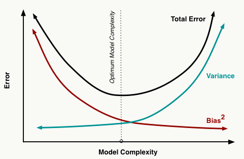
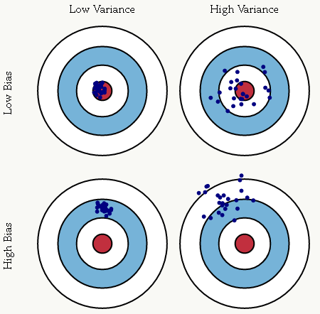
2.0 偏差与方差 在机器学习算法中,偏差是由先验假设的不合理带来的模型误差,高偏差会导致欠拟合 : 所谓欠拟合是指对特征和标注之间的因果关系学习不到位,导致模型本身没有较好的学到历史经验的现象; 方差表征的是模型误差对样本发生一定变化时的敏感度,高方差会导致过拟合 :模型对训练样本中的随机噪声也做了拟合学习,导致在未知样本上应用时出现效果较差的现象; 机器学习模型的核心之一在于其推广能力,即在未知样本上的表现。 对方差和偏差的一种直观解释:
一个例子,假如我们有预测模型:
\[ \begin{array}{l} y=f(x)+\epsilon\\ \epsilon \sim N(0,\sigma) \end{array} \]
我们希望用 \(f^{e}(x)\) 估计 \(f(x)\) ,如果使用基于square loss 的线性回归,则误差分析如下: \[ \begin{align*} Err(x)&=E[(y-f^{e}(x))^2]\\ &=E[(f(x)-f^{e}(x))^2]+\sigma_e^2\\ &=[f(x)]^2-2f(x)E[f^{e}(x)]+E[f^{e}(x)^2]+\sigma_e^2\\ &=E[f^{e}(x)]^2-2f(x)E[f^{e}(x)]+[f(x)]^2\\ &+E[f^{e}(x)^2]-2E[f^{e}(x)]^2+E[f^{e}(x)]^2+\sigma_e^2\\ &=E[f^{e}(x)]^2-2f(x)E[f^{e}(x)]+[f(x)]^2\\ &+E[f^{e}(x)^2-2f^{e}(x)E[f^{e}(x)]+E[f^{e}(x)]^2]+\sigma_e^2\\ &=\underbrace{(E[f^{e}(x)]-f(x))^2}_{Bias^2}+\underbrace{E[(f^{e}(x)-E[f^{e}(x)])^2]}_{Variance}+\sigma_e^2\\ \end{align*} \]
所以大家可以清楚的看到模型学习过程其实就是对偏差和方差的折中过程。
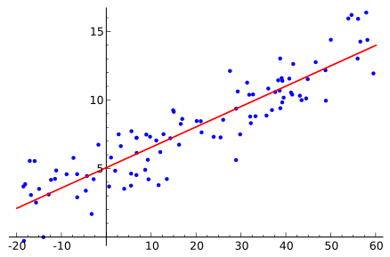
2.1 线性回归-Linear Regression 简单线性回归 2.1.1 模型原理 标准线性回归通过对自变量的线性组合来预测因变量,组合自变量的权重通过最小化训练集中所有样本的预测平方误差和来得到,原理如下。
\[ \tilde y_i=\sum_{i=1}^N w^Tx_i\]
\[min~\frac{1}{2}\sum_{i=1}^N(y_i-\tilde y_i)^2\]
所有机器学习模型的成立都会有一定的先验假设,线性回归也不例外,它对数据做了以下强假设:
自变量相互独立,无多重共线性
因变量是自变量的线性加权组合:
\[y=w^Tx+\epsilon\]
所有样本独立同分布(iid),且误差项服从以下分布: \[\epsilon \sim N(0,\sigma^2)\]
最小二乘法与以上假设的关系推导如下: \[ \begin{array}{l} \because y=w^Tx+\epsilon,~~~~~\epsilon \sim N(0,\sigma^2)\\ \therefore p(y|x) = N(w^Tx,\sigma^2)\\ \Rightarrow p(y|x) = \frac{1}{\sqrt {2\pi}\sigma} e^{-\frac{(y-w^Tx)^2}{2\sigma^2}} \end{array} \]
使用MLE(极大似然法)估计参数如下: \[ \begin{array}{l} w=arg~max_w\sum_{i=1}^Nlog~p(y_i|x_i)\\ \Leftrightarrow w=arg~min_w\frac{1}{2}\sum_{i=1}^N{(y_i-w^Tx_i)^2} \end{array} \]
线性回归有两个重要变体:
Lasso Regression:采用L1正则并使用MAP做参数估计 Ridge Regression:采用L2正则并使用MAP做参数估计 关于正则化及最优化后续会做介绍。
2.1.2 损失函数 损失函数1 —— Least Square Loss
\[loss(x)=\frac{1}{2}\sum_{i=1}^N(y_i-\tilde y_i)^2\]
进一步阅读可参考:Least Squares
Q: 模型和损失的关系是什么?
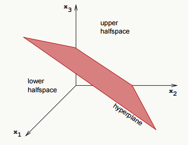
2.2 支持向量机-Support Vector Machine 支持向量机通过寻找一个分类超平面使得(相对于其它超平面)它与训练集中任何一类样本中最接近于超平面的样本的距离最大。虽然从实用角度讲(尤其是针对大规模数据和使用核函数)并非最优选择,但它是大家理解机器学习的最好模型之一,涵盖了类似偏差和方差关系的泛化理论、最优化原理、核方法原理、正则化等方面知识。
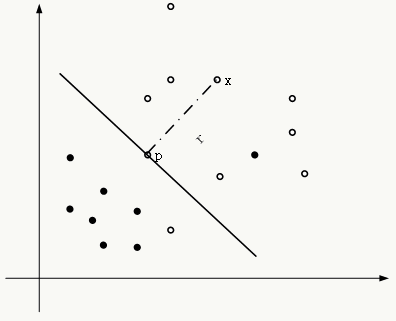
2.2.1 模型原理 SVM原理可以从最简单的解析几何问题中得到:
超平面的定义如下: \[ \begin{array}{l} y=f(x)=w^Tx+b\\ f(x)=0 \end{array} \]
从几何关系上来看,超平面与数据点的关系如下(以正样本点为例): \[ \begin{array}{l} x_i=p_i+\gamma_i\frac{w}{\Arrowvert w\Arrowvert}\\ \text{where the p is point x's projection on the hyperplane.}\\ \Leftrightarrow w^Tx_i+b=w^Tp_i+b+\gamma_i\frac{w^Tw}{\Arrowvert w\Arrowvert}\\ \because f(p_i)=0\\ \therefore f(x_i)=\gamma_i\Arrowvert w\Arrowvert\\ \Rightarrow \gamma_i=\frac{f(x_i)}{\Arrowvert w\Arrowvert}\\ \text{consider two cases(label=}\pm1\text{)}\\ \Rightarrow \gamma_i=\frac{y_if(x_i)}{\Arrowvert w\Arrowvert}\\ \text{set}~~\tilde{\gamma_i}=y_if(x_i)\\ \Rightarrow \gamma_i=\frac{\tilde{\gamma_i}}{\Arrowvert w\Arrowvert} \end{array} \]
定义几何距离和函数距离分别如下: \[ \begin{array}{l} \text{relative geometric margin:}~~~~\tilde{\gamma}=min_1^N\tilde{\gamma_i}\\ \text{relative functional margin:}~~~~\gamma=min_1^N\gamma_i \end{array} \]
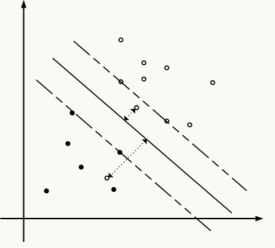
由于超平面的大小对于SVM求解并不重要,重要的是其方向,所以根据SVM的定义,得到约束最优化问题: \[ \begin{array}{l} max~~\gamma\\ ~~~st.~y_i\frac{f(x_i)}{\Arrowvert w\Arrowvert}\ge \gamma,~~i=1,2....N\\ \Leftrightarrow \\ max~\frac{\tilde{\gamma}}{\Arrowvert w\Arrowvert}\\ ~~~st.~y_if(x_i)\ge \tilde{\gamma},~~i=1,2....N\\ \text{the value of } \tilde{\gamma}\text{ does not affect the solution of the problem.}\\ \text{to set } \tilde{\gamma}=1.\\ \Leftrightarrow \\ min~\frac{1}{2}\Arrowvert w\Arrowvert^2\\ ~~~st.~y_if(x_i)-1\ge 0,~~i=1,2....N\\ \end{array} \]
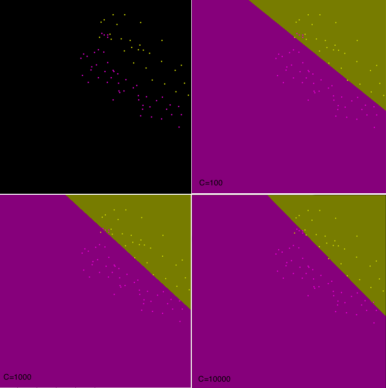
现实当中我们无法保证数据是线性可分的,强制要求所有样本能正确分类是不太可能的,即使做了核变换也只是增加了这种可能性,因此我们又需要做折中,允许误分的情况出现,对误分的样本根据其严重性做惩罚,所以引入松弛变量,将上述问题变成软间隔优化问题。
新的优化问题: \[ \begin{align*} min&~\frac{1}{2}\Arrowvert w\Arrowvert^2+C\sum_{i=1}^Ng(\xi_i)\\ st.&~y_if(x_i)\ge 1-\xi_i,~~i=1,2....N\\ &\xi_i\ge 0,~~i=1,2....N\\ &g(\xi)=\xi \text{ or } g(\xi)=\xi^2.....\\ \end{align*} \]
如果选择: \[g(\xi)=\xi\]
那么优化问题变成: \[ \begin{array}{l} min~\frac{1}{2}\Arrowvert w\Arrowvert^2+C\sum_{i=1}^N\xi_i\\ ~~~st.~y_if(x_i)\ge 1-\xi_i,~~i=1,2....N\\ ~~~~~~~~~\xi_i\ge 0,~~i=1,2....N\\ \end{array} \]
2.2.2 损失函数 损失函数2 —— Hinge Loss
\[loss(x)=\sum_{i=1}^N[1-y_if(x_i)]_+\]
使用hinge loss将SVM套入机器学习框架,让它更容易理解。此时原始约束最优化问题变成损失函数是hinge loss且正则项是L2正则的无约束最优化问题:
\[ \begin{array}{l} (1)min~\frac{1}{2}\Arrowvert w\Arrowvert^2+C\sum_{i=1}^N\xi_i\\ ~~~st.~y_if(x_i)\ge 1-\xi_i,~~i=1,2....N\\ ~~~~~~~~~\xi_i\ge 0,~~i=1,2....N\\ \Leftrightarrow \\ (2)min~\sum_{i=1}^N[1-y_if(x_i)]_++\lambda \Arrowvert w\Arrowvert^2 \end{array} \]
下面我证明以上问题(1)和问题(2)是等价的(反之亦然):
\[ \begin{array}{l} && \because 1-y_if(x_i)\leq \xi_i \text{ and }0 \leq \xi_i\\ && \text{if }1-y_if(x_i)\geq 0 \text{ then}\\ && ~~~~min~\frac{1}{2}\Arrowvert w\Arrowvert^2+C\sum_{i=1}^N\xi_i\\ && ~~~~\Leftrightarrow \\ && ~~~~min~\frac{1}{2}\Arrowvert w\Arrowvert^2+C\sum_{i=1}^N1-y_if(x_i)\\ && \text{if }1-y_if(x_i)<0\text{ then}\\ && ~~~~min~\frac{1}{2}\Arrowvert w\Arrowvert^2+C\sum_{i=1}^N\xi_i\\ && ~~~~\Leftrightarrow \\ && ~~~~min~\frac{1}{2}\Arrowvert w\Arrowvert^2\\ && \therefore\\ && min~\frac{1}{2}\Arrowvert w\Arrowvert^2+C\sum_{i=1}^N\xi_i\\ && ~~~st.~y_if(x_i)\ge 1-\xi_i,~~i=1,2....N\\ && ~~~~~~~~~\xi_i\ge 0,~~i=1,2....N\\ \Leftrightarrow \\ && min~\sum_{i=1}^N[1-y_if(x_i)]_++\lambda \Arrowvert w\Arrowvert^2\\ \end{array} \]
到此为止,SVM和普通的判别模型没什么两样,也没有support vector的概念,它之所以叫SVM就得说它的对偶形式了,通过拉格朗日乘数法对原始问题做对偶变换:
\[ \begin{align*} min&~\frac{1}{2}\Arrowvert w\Arrowvert^2+C\sum_{i=1}^N\xi_i\\ st.&~y_if(x_i)\ge 1-\xi_i,~~i=1,2....N\\ &~\xi_i\ge 0,~~i=1,2....N\\ \Rightarrow& \\ &L(w,b,\xi,\alpha,\mu)=\frac{1}{2}\Arrowvert w\Arrowvert^2+C\sum\limits_{i=1}^{N}\xi_i\\ &-\sum\limits_{i=1}^{N}\alpha_i(y_i(w^Tx_i+b)-1+\xi_i)-\sum\limits_{i=1}^{N}\mu_i\xi_i\\ &\text{(KKT conditions)}\\ &\frac{\partial{L}}{\partial{w}}=w-\sum\limits_{i=1}^{n}y_i\alpha_i x_i=0\\ &\frac{\partial{L}}{\partial{b}}=\sum\limits_{i=1}^{n}y_i\alpha_i=0\\ &\frac{\partial L}{\partial \xi}=C-\alpha-\mu=0\\ &\text{(Complementary Slackness condition)}\\ &\alpha_i(y_i(w^Tx_i+b)- 1+\xi_i)=0\\ &\mu_i\xi_i=(\alpha_i-C)\xi_i=0\\ &\alpha_i\geq 0\\ &\xi_i\geq 0\\ &\mu_i\geq 0\\ &\text{(Replace inner product with the kernel function)}\\ \\ &\Rightarrow \\ max&~\sum\limits_{i=1}^{N}\alpha_i-\frac{1}{2}\sum\limits_{i,j=1}^{N}{y_iy_j\alpha_i\alpha_j(K(x_i,x_j))}\\ st.&~\sum\limits_{i=1}^{n}y_i\alpha_i=0\\ &0 \leq \alpha_i \leq C\\ \end{align*} \]
从互补松弛条件可以得到以下信息:
当\(\alpha_i=C\) 时,松弛变量\(\xi_i\) 不为零,此时其几何间隔小于\(1/\Arrowvert w\Arrowvert\) ,对应样本点就是误分点;当\(\alpha_i=0\) 时,松弛变量\(\xi_i\) 为零,此时其几何间隔大于\(1\Arrowvert w\Arrowvert\) ,对应样本点就是内部点,即分类正确而又远离最大间隔分类超平面的那些样本点;而\(0 < \alpha_i <C\) 时,松弛变量\(\xi_i\) 为零,此时其几何间隔等于\(1/ \Arrowvert w\Arrowvert\) ,对应样本点 就是支持向量 。\(\alpha_i\) 的取值一定是\([0,C]\) ,这意味着向量\(\alpha\) 被限制在了一个边长为\(C\) 的盒子里。 详细说明可参考:SVM学习——软间隔优化 。
\(C\) 越大表明你越不想放弃离群点,分类超平面越向离群点移动当以上问题求得最优解\(\alpha^*\) 后,几何间隔变成如下形式: \[\gamma=(\sum\limits_{i,j \in \{support~vectors\}}y_iy_j\alpha_i^*\alpha_j^*K(x_i,x_j))^{-1/2}\] 它只与有限个样本有关系,这些样本被称作支持向量,从这儿也能看出此时模型参数个数与样本个数有关系,这是典型的非参学习过程。
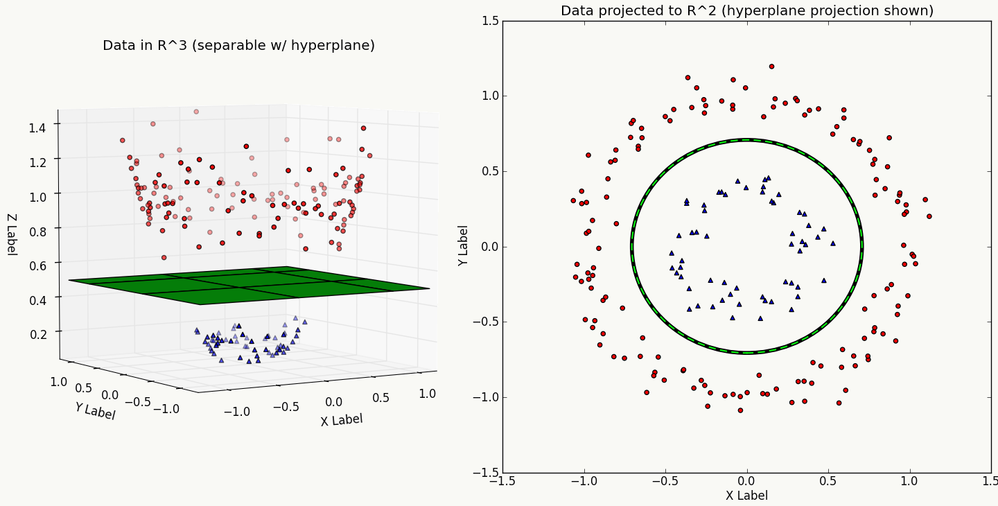
2.2.3 核方法 上面对将内积\(x_i^Tx_j\) 用一个核函数\(K(x_i,x_j)\) 做了代替,实际上这种替换不限于SVM,所有出现样本间内积的地方都可以考虑这种核变换,本质上它就是通过某种隐式的空间变换在新空间(有限维或无限维兼可)做样本相似度衡量,采用核方法后的模型都可以看做是无固定参数的基于样本的学习器,属于非参学习,核方法与SVM这类模型的发展是互相独立的。
from Kernel Trick 这里不对原理做展开,可参考:
1、Kernel Methods for Pattern Analysis
2、the kernel trick for distances
一些可以应用核方法的模型:
SVM Perceptron PCA Gaussian processes Canonical correlation analysis Ridge regression Spectral clustering 在我看来核方法的意义在于: 1、对样本进行空间映射,以较低成本隐式的表达样本之间的相似度,改善样本线性可分的状况,但不能保证线性可分; 2、将线性模型变成非线性模型从而提升其表达能力,但这种升维的方式往往会造成计算复杂度的上升。
一些关于SVM的参考资料:
SVM学习——线性学习器
SVM学习——求解二次规划问题
SVM学习——核函数
SVM学习——统计学习理论
SVM学习——软间隔优化
SVM学习——Coordinate Desent Method
SVM学习——Sequential Minimal Optimization
SVM学习——Improvements to Platt’s SMO Algorithm
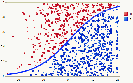
2.3 逻辑回归-Logistic Regression 逻辑回归恐怕是互联网领域用的最多的模型之一了,很多公司做算法的同学都会拿它做为算法系统进入模型阶段的baseline。
2.3.1 模型原理 逻辑回归是一种判别模型,与线性回归类似,它有比较强的先验假设 :
\[ \begin{align*} p(y|x)&=Bernoulli(\pi)\\ &=p(y=1|x)^y(1-p(y=1|x))^{1-y},y\in\{0,1\} \end{align*} \]
\[p(x_i|y=y_k)=Gaussian(\mu_{ik},\sigma_i)\]
\(y\) 是样本标注,布尔类型,取值为0或1;
\(x\) 是样本的特征向量。
逻辑回归是判别模型,所以我们直接学习\(p(y|x)\) ,以高斯分布为例:
\[p(y=1|x)=\frac{1}{1+e^{-(w^Tx+b)}}\]
\[p(y=0|x)=\frac{1}{1+e^{(w^Tx+b)}}\]
整个原理部分的推导过程如下:
\[ \begin{align*} p(y=1|x)&=\frac{p(x|y=1)p(y=1)}{p(x)}\\ &=\frac{p(x|y=1)p(y=1)}{p(x|y=1)p(y=1)+p(x|y=0)p(y=0)}\\ &=\frac{1}{1+\frac{p(x|y=0)p(y=0)}{p(x|y=1)p(y=1)}}\\ &=\frac{1}{1+\frac{p(x|y=0)(1-p(y=1))}{p(x|y=1)p(y=1)}}~~\text {to set p(y=1)=}\pi\\ &=\frac{1}{1+\frac{p(x|y=0)(1-\pi)}{p(x|y=1)\pi}}\\ &=\frac{1}{1+e^{ln\frac{1-\pi}{\pi}+ln\frac{p(x|y=0)}{p(x|y=1)}}}\\ &=\frac{1}{1+e^{ln\frac{1-\pi}{\pi}+\sum_iln\frac{p(x_i|y=0)}{p(x_i|y=1)}}}\\ \end{align*} \] \[ \begin{align*} &\because p(x_i|y_k)=\frac{1}{\sigma_{ik}\sqrt{2\pi}}e^{-\frac{(x_i-\mu_{ik})^2}{2\sigma_{ik}^2}}\\ &\therefore p(y=1|x)=\frac{1}{1+e^{-(ln\frac{\pi-1}{\pi}+\sum_i(\frac{\mu_{i1}-\mu_{i0}}{\sigma_i^2}x_i+\frac{\mu_{i0}^2-\mu_{i1}^2}{2\sigma_i^2}))}}\\ &\qquad\qquad\qquad =\frac{1}{1+e^{-(\sum_iw_ix_i+b)}},i=1,2,...,dim\\ &\text{where}\\ &\qquad\qquad\qquad b=\sum_i\frac{\mu_{i0}^2-\mu_{i1}^2}{2\sigma_i^2}+ln\frac{\pi-1}{\pi}\\ &\qquad\qquad\qquad w_i=\frac{\mu_{i1}-\mu_{i0}}{\sigma_i^2} \end{align*} \]
采用 MLE 或者 MAP 做参数求解:
\[ \begin{array}{l} w=arg~max_w\sum_{i=1}^Nln~p(y_i|x_i)\\ \Leftrightarrow \\ w=arg~min_w\sum_{i=1}^N{y_iln~p(y_i=1|x_i)+(1-y_i)ln~p(y_i=0|x_i)} \end{array} \]
2.3.2 损失函数 损失函数3 —— Cross Entropy Loss
\[ \begin{array}{l} loss(x)=H_p(q)=\sum_{i=1}^N\sum_y(\int_y) p(y|x_i)ln\frac{1}{q(y|x_i)}\\ \text{especially for bernoulli distribution:}\\ loss(x)=\sum_{i=1}^Ny_i ln ~p(y_i|x_i)+(1-y_i)(1-ln~p(y_i|x_i)) \end{array} \]
简单理解,从概率角度:Cross Entropy损失函数衡量的是两个概率分布\(p\) 与\(q\) 之间的相似性,对真实分布估计的越准损失越小;从信息论角度:用编码方式\(q\) 对由编码方式\(p\) 产生的信息做编码,如果两种编码方式越接近,产生的信息损失越小。与Cross Entropy相关的一个概念是Kullback–Leibler divergence,后者是衡量两个概率分布接近程度的标量值,定义如下: \[D_q(p) = \sum_x(\int_x) p(x)\log_2\left(\frac{p(x)}{q(x)} \right)\] 当两个分布完全一致时其值为0,显然Cross Entropy与Kullback–Leibler divergence的关系是: \[H_p(q)=H(p)+D_q(p)\]
关于交叉熵及其周边原理,有一篇文章写得特别好:Visual Information Theory
2.4 Bagging and Boosting框架 Bagging和Boosting是两类最常用以及好用的模型融合框架,殊途而同归。
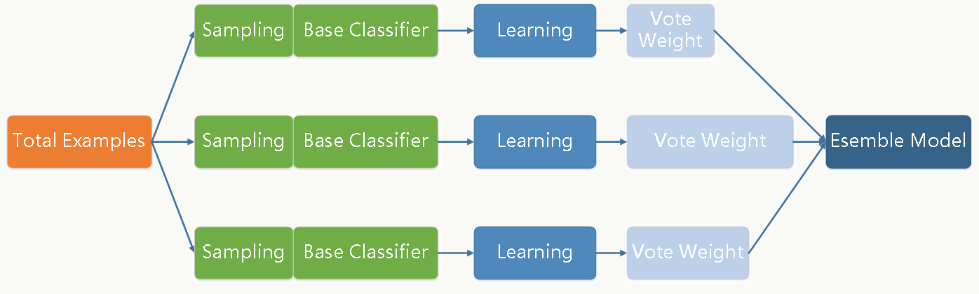
2.4.1 Bagging框架 Bagging(Breiman, 1996) 方法是通过对训练样本和特征做有放回的抽样,并拟合若干个基础模型进而通过投票方式做最终分类决策的框架。每个基础分类器(可以是树形结构、神经网络等等任何分类模型)的特点是
低偏差、高方差 ,框架通过(加权)投票方式降低方差,使得整体趋于
低偏差、低方差 。
分析如下:
假设任务是学习一个模型 \(y=f(x)\) ,我们通过抽样生成生成\(N\) 个数据集,并训练得到\(N\) 个基础分类器\(c_i......c_N\) 。
\[ \begin{array}{l} \text{define}:\\ \qquad\qquad (1). y=f(x), \text{prediction function}\\ \qquad\qquad (2). o_i(x)=c_i(x), \text{ $c_i$ is the i-th classifier}\\ \qquad\qquad (3). \overline{o}(x)=\sum_{i=1}^Nw_io_i(x), \text{ where } \sum_{i=1}^Nw_i=1\\ \qquad\qquad (4). v_i(x)=[o_i(x)-\overline{o}(x)]^2\\ \qquad\qquad (5). \overline{v}(x)=\sum_{i=1}^Nw_iv_i(x)=\sum_{i=1}^Nw_i[o_i(x)-\overline{o}(x)]^2\\ \qquad\qquad (6). \overline{\epsilon}(x)=\sum_{i=1}^Nw_i[(f(x)-o_i(x))^2]\\ \qquad\qquad 7). e(x)=(f(x)-\overline{o}(x))^2 \\ \because \overline{v}(x)=\sum_{i=1}^Nw_i[o_i(x)-\overline{o}(x)]^2\\ \qquad\qquad =\sum_{i=1}^Nw_i[(f(x)-o_i(x))-(f(x)-\overline{o}(x))]^2\\ \qquad\qquad =\sum_{i=1}^Nw_i[(f(x)-o_i(x))^2+(f(x)-\overline{o}(x))^2\\ \qquad\qquad -2(f(x)-o_i(x))(f(x)-\overline{o}(x))]\\ \qquad\qquad =\sum_{i=1}^Nw_i[(f(x)-o_i(x))^2]-(f(x)-\overline{o}(x))^2\\ \therefore e(x)=\overline{\epsilon}(x)-\overline{v}(x) \end{array} \]
从结论可以发现多分类器投票机制的引入可以降低模型方差从而降低分类错误率,大家可以多理解理解这一系列推导。
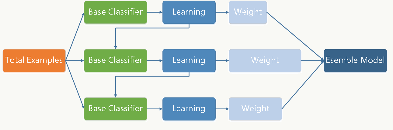
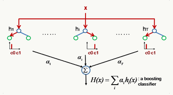
2.4.2 Boosting框架 Boosting(Freund & Shapire, 1996) 通过迭代方式训练若干基础分类器,每个分类器依据上一轮分类器产生的残差做权重调整,每轮的分类器需要够“简单”,具有
高偏差、低方差 的特点,框架再辅以(加权)投票方式降低偏差,使得整体趋于
低偏差、低方差 。
一个简单的总结: \[ \begin{array}{l} F(x)=\sum_{i=1}^Nw_if_i(x)\\ \text{where:}\\ \qquad f_i\text{ is the base classier }i\\ \qquad w_i \text{ is the weight of classier }i\\ \qquad x \text{ is the feature vector of example}\\ \text{define:}\\ \qquad \text{(1). margin of an example(x,y) with respect to the classier is yF(x)}\\ \qquad \text{(2). cost function of $N$ examples is $C(F)=\frac{1}{N}\sum_{i=1}^NC(y_iF(x_i))$}\\ \text{Now we wish to find a new $f$ to add to F so that $C(F+\alpha f)$ can be decreased}\\ \because C(F+\alpha f)=C(F)+\alpha\langle\nabla{C(F)},f\rangle\\ \therefore \text{the greatest reduction of $C$ will satisfied: }\\ \qquad\qquad\qquad f=Max~-\langle\nabla{C(F)},f\rangle \end{array} \]
AnyBoost Algorithm
Boost算法是个框架,很多模型都能往进来套。 \[ \begin{array}{l} F_0(x)=0\\ \text{for $i$=0 to T:}\\ \qquad f_{t+1}=classifier(F_t)\\ \qquad if~~-\langle\nabla{C(F)},f_{t+1}\rangle \le0:\\ \qquad\qquad return~F_t\\ \qquad choose~w_{t+1}\\ \qquad F_{t+1}=F_t+w_{t+1}f_{t+1}\\ return~F_{T+1} \end{array} \]
Q: boosting 和 margin的关系是什么(机器学习中margin的定义为\(yf(x)\) )?
Q: 类似bagging,为什么boosting能够通过reweight及投票方式降低整体偏差?
2.5 Additive Tree 模型 Additive tree models (ATMs)是指基础模型是树形结构的一类融合模型,可做分类、回归,很多经典的模型可以被看做ATM模型,比如Random forest 、Adaboost with trees、GBDT等。
ATM 对N棵决策树做加权融合,其判别函数为:
\[ \begin{array}{l} F(x)=\sum_{i=1}^Nw_if_i(x)\\ \text{where }f_i\text{ is the output of tree }i\\ \qquad\qquad\qquad w_i \text{ is the weight of tree }i\\ \qquad\qquad\qquad x \text{ is the feature vector of instance} \end{array} \]
2.5.1 Random Forests Random Forest 属于bagging类模型,每棵树会使用各自随机抽样样本和特征被独立的训练。
\[ \begin{array}{l} \text{for $t$ = 1 to $T$:}\\ \qquad \text{(1). Sample $n$ instances from the dataset with replacement}\\ \qquad \text{(2). Randomization:}\\ \qquad \qquad\text{$\bullet$ Bootstrap samples.}\\ \qquad \qquad\text{$\bullet$ Random selection of $K\le p$ split variables.}\\ \qquad \qquad\text{$\bullet$ Random selection of threshold.}\\ \qquad \text{(2). Train an low-bias unpruned decision or regression tree $f_t$ on the sampled instances }\\ \\ \text{The final is the average of the outputs from all the trees:}\\ F(x)=\sum_{i=1}^Tw_if_i(x)\\ ~~~where~\sum_{i=1}^Tw_i=1,~(such~ as ~w_i=\frac{1}{T}) \end{array} \]
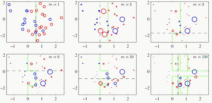
2.5.2 AdaBoost with trees AdaBoost with trees通过训练多个弱分类器来组合得到一个强分类器,每次迭代会生成一棵高偏差、低方差 的树形弱分类器,每一轮的训练会更关注上一轮被分类器分错的样本,为其加大权重,训练过程如下:
\[ \begin{array}{l} f_0(x)=0\\ \text{for $i$=1 to $T$:}\\ \qquad minimize~\sum_{i=1}^NL(y_i,F_t(x_i)+\alpha_tf_t(x_i))\\ \qquad F_{t+1}(x)=F_t(x)+\alpha_tf_t(x)\\ \\ \text{The final is weighted average of the outputs from all the weak classifiers:}\\ F(x)=\sum_{i=1}^T\alpha_if_i(x)\\ \end{array} \]
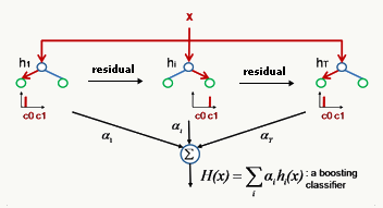
From Bishop(2006) 2.5.3 Gradient Boosting Decision Tree Gradient boosted 是一类boosting的技术,不同于Adaboost加大误分样本权重的策略,它每次迭代加的是上一轮梯度更新值: \[\sum_{i=1}^NL(y_i,F_t(x_i)+\alpha_tf_t(x_i))\]
其训练过程如下:
\[ \begin{array}{l} F_{t+1}(x)=F_t(x)+\alpha_tf_t(x)\\ f_t(x_i)\thickapprox -\frac{\partial L(y_i,F_t(x_i))}{\partial F_t(x_i)}\\ \qquad \text{where $\alpha_t$ is the learning rate.} \end{array} \]
GBDT是基础分类器为决策树的可做分类和回归的模型。
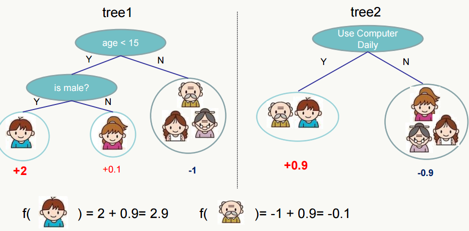
目前我认为最好的GBDT的实现是XGBoost: 其回归过程的示例图如下,通过对样本落到每棵树的叶子节点的权重值做累加来实现回归(或分类):
Regression Tree Ensemble from chentianqi 其原理推导如下:
\[ \begin{array}{l} \text{Prediction model: }F(x)=\sum_{i=1}^Tw_if_i(x)\\ \text{Objective: }obj^t=\sum_{i=1}^NL(y_i,F_i^t(x_i))+\Omega(f_t)\\ \qquad \text{where N is instance numbers and t is current trees.}\\ \because obj^t=\sum_{i=1}^NL(y_i,F_i^t(x_i))+\Omega(f_t)\\ \qquad =\sum_{i=1}^NL(y_i,F_i^{t-1}(x_i)+w_tf_t(x_i))+\Omega(f_t)\\ \text{Recall: }f(x+\Delta x)\thickapprox f(x)+\nabla f(x)\Delta x+\frac{1}{2}\nabla^2 f(x)\Delta x^2\\ \therefore obj^t\thickapprox\sum_{i=1}^N[L(y_i,F_i^{t-1}(x_i))+\nabla _{F_{t-1}}L(y_i,F_i^{t-1}(x_i))w_tf_t(x_i)\\ \qquad \qquad \frac{1}{2}\nabla _{F_{t-1}}^2L(y_i,F_i^{t-1}(x_i))w_t^2f_t^2(x_i)]+\Omega(f_t)\\ \text{set $g_i=\nabla _{F_{t-1}}L(y_i,F_i^{t-1}(x_i))$}\\ \qquad h_i=\nabla _{F_{t-1}}^2L(y_i,F_i^{t-1}(x_i))\\ \qquad obj^t\thickapprox \sum_{i=1}^N[L(y_i,F_i^{t-1}(x_i))+g_iw_tf_t(x_i)+\frac{1}{2}h_iw_t^2f_t^2(x_i)]+\Omega(f_t)\\ \because L(y_i,F_i^{t-1}(x_i)) \text{ is constant.}\\ \therefore \text{Our objective function is:}\\ \qquad obj^t=\sum_{i=1}^N[g_iw_tf_t(x_i)+\frac{1}{2}h_iw_t^2f_t^2(x_i)]+\Omega(f_t)+C\\ \text{Define tree by a vector of scores in leafs,any instance will be mapped to a leaf:}\\ f_t(x)=m_q(x),~~m\in R^T,~~q:R^d\rightarrow\{1,2,3,...,T\}\\ \Omega(f_t)=\gamma T+ \frac{1}{2}\lambda \sum_{i=1}^Tm_j^2,\\ \text{where $T$ is total number of leaf nodes of $t$ trees}\\ \qquad \qquad \text{$m_j$ is the weight of j-th leaf node.}\\ \text{Define the instance set in leaf $j$ as $I_j=\{i|j=q(x_i)\}$}\\ \text{Our new objective function is:}\\ obj^t=\sum_{i=1}^N[g_iw_tf_t(x_i)+\frac{1}{2}h_iw_t^2f_t^2(x_i)]+\Omega(f_t)\\ \qquad =\sum_{i=1}^N[g_iw_tm_q(x_i)+\frac{1}{2}h_iw_t^2m_q^2(x_i)]+\gamma T+ \frac{1}{2}\lambda \sum_{i=1}^Tm_j^2\\ \qquad =\sum_{j=1}^T[(\sum_{i \in I_j}g_i)w_tm_j+\frac{1}{2}(\sum_{i \in I_j}h_iw_t^2+\lambda )m_j^2]+\gamma T\\ \text{Define $G_j=\sum_{i \in I_j}g_i$ and $H_j=\sum_{i \in I_j}h_i$ then}\\ obj^t=\sum_{j=1}^T[G_jw_tm_j+\frac{1}{2}(H_jw_t^2+\lambda)m_j^2]+\gamma T\\ \text{For a quadratic function optimization problems:}\\ m_j^*=-\frac{G_j^2w_t}{H_jw_t^2+\lambda}\\ obj^*=-\frac{1}{2}\sum_{j=1}^T\frac{G_j^2w_t^2}{H_jw_t^2+\lambda}+\gamma T\\ \text{If we set $w_t=1$ then}\\ m_j^*=-\frac{G_j}{H_j+\lambda}\\ obj^*=-\frac{1}{2}\sum_{j=1}^T\frac{G_j^2}{H_j+\lambda}+\gamma T\\ \text{So when we add a split, our obtained gain is:}\\ gain=\underbrace{\frac{G_L^2}{H_L+\lambda}}_{left ~child}+\underbrace{\frac{G_R^2}{H_R+\lambda}}_{right~child}-\underbrace{\frac{(G_L+G_R)^2}{H_L+H_R+\lambda}}_{do~not~split}-\gamma~~~~(thinking~why?) \end{array} \]
对GBDT来说依然避免不了过拟合,所以与传统机器学习一样,通过正则化策略可以降低这种风险:
通过观察模型在验证集上的错误率,如果它变化不大则可以提前结束训练,控制迭代轮数(即树的个数);
\(F_{t+1}(x)=F_t(x)+\alpha_tf_t(x)\) 从迭代的角度可以看成是学习率(learning rate),从融合(ensemble)的角度可以看成每棵树的权重,\(\alpha\) 的大小经验上可以取0.1,它是对模型泛化性和训练时长的折中;
借鉴Bagging的思想,GBDT可以在每一轮树的构建中使用训练集中无放回抽样的样本,也可以对特征做抽样,模拟真实场景下的样本分布波动;
\(\Omega(f_t)=\gamma T+ \frac{1}{2}\lambda \sum_{i=1}^Tm_j^2\) 通过对树的叶子节点个数、叶子节点权重做显式的正则化达到缓解过拟合的效果;
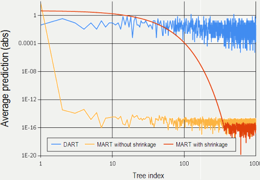
模拟深度学习里随机放弃更新权重的方法,可以在每新增一棵树的时候拟合随机抽取的一些树的残差,相关方法可以参考:
DART: Dropouts meet Multiple Additive Regression Trees ,文中对该方法和Shrinkage的方法做了比较:
XGBoost源码在: https://github.com/dmlc中,其包含非常棒的设计思想和实现,建议大家都去学习一下,一起添砖加瓦。原理部分我就不再多写了,看懂一篇论文即可,但特别需要注意的是文中提到的weighted quantile sketch 算法,它用来解决当样本集权重分布不一致时如何选择分裂节点的问题:XGBoost: A Scalable Tree Boosting System 。
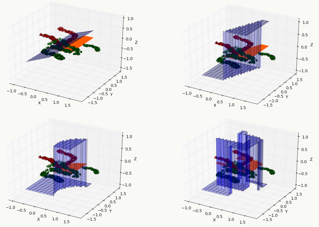
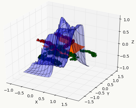
2.5.4 简单的例子 下面是关于几个常用机器学习模型的对比,从中能直观地体会到不同模型的运作区别,数据集采用libsvm作者整理好的fourclass_scale数据集,机器学习工具采用sklearn,代码中模型未做任何调参,仅使用默认参数设置。
1
2
3
4
5
6
7
8
9
10
11
12
13
14
15
16
17
18
19
20
21
22
23
24
25
26
27
28
29
30
31
32
33
34
35
36
37
38
39
40
41
42
43
44
45
46
47
48
49
50
51
52
53
54
55
56
57
58
59
60
61
62
63
64
65
66
67
68
69
70
71
72
73
74
75
76
77
78
79
80
81
82
83
84
85
86
87
88
89
90
91
92
93
94
95
96
97
98
99
100
101
102
103
104
105
106
107
108
109
110
111
112
113
114
115
116
117
118
119
120
121
122
123
import urllibimport matplotlibimport osmatplotlib.use('Agg' ) from matplotlib import pyplot as pltfrom mpl_toolkits.mplot3d import proj3dimport numpy as npfrom mpl_toolkits.mplot3d import Axes3Dfrom sklearn.externals.joblib import Memoryfrom sklearn.datasets import load_svmlight_filefrom sklearn import metricsfrom sklearn.metrics import roc_auc_scorefrom sklearn import svmfrom sklearn.linear_model import LogisticRegressionfrom sklearn.linear_model import Ridgefrom sklearn.ensemble import GradientBoostingClassifierfrom mpl_toolkits.mplot3d import Axes3Dfrom matplotlib import cmfrom matplotlib.ticker import LinearLocator, FormatStrFormatterfrom sklearn.tree import DecisionTreeClassifierimport kerasfrom keras.models import Sequentialfrom keras.layers.core import Dense,Dropout,Activationdef download (outpath ): filename=outpath+"/fourclass_scale" if os.path.exists(filename) == False : urllib.urlretrieve("https://www.csie.ntu.edu.tw/~cjlin/libsvmtools/datasets/binary/fourclass_scale" ,filename) def data_building (): dtrain = load_svmlight_file('fourclass_scale' ) train_d=dtrain[0 ].toarray() train_l=dtrain[1 ] x1 = train_d[:,0 ] x2 = train_d[:,1 ] y = train_l px1 = [] px2 = [] pl = [] nx1 = [] nx2 = [] nl = [] idx = 0 for i in y: if i == 1 : px1.append(x1[idx]-0.5 ) px2.append(x2[idx]+0.5 ) pl.append(i) else : nx1.append(x1[idx]+0.8 ) nx2.append(x2[idx]-0.8 ) nl.append(i) idx = idx + 1 x_axis, y_axis = np.meshgrid(np.linspace(x1.min (), x1.max (), 100 ), np.linspace(x2.min (), x2.max (), 100 )) return x_axis, y_axis, px1, px2, nx1, nx2, train_d, train_l def paint (name, x_axis, y_axis, px1, px2, nx1, nx2, z ): fig = plt.figure() ax = Axes3D(fig) ax=plt.subplot(projection='3d' ) ax.scatter(px1,px2,c='r' ) ax.scatter(nx1,nx2,c='g' ) ax.plot_surface(x_axis, y_axis,z.reshape(x_axis.shape), rstride=8 , cstride=8 , alpha=0.3 ) ax.contourf(x_axis, y_axis, z.reshape(x_axis.shape), zdir='z' , offset=-100 , cmap=cm.coolwarm) ax.contourf(x_axis, y_axis, z.reshape(x_axis.shape), levels=[0 ,max (z)], cmap=cm.hot) ax.set_xlabel('X' ) ax.set_ylabel('Y' ) ax.set_zlabel('Z' ) fig.savefig(name+".png" , format ='png' ) def svc (x_axis, y_axis, x,y ): clf = svm.SVC() clf.fit(x, y) y = clf.predict(np.c_[x_axis.ravel(), y_axis.ravel()]) return y def lr (x_axis, y_axis, x,y ): clf = LogisticRegression() clf.fit(x, y) y = clf.predict(np.c_[x_axis.ravel(), y_axis.ravel()]) return y def ridge (x_axis, y_axis, x,y ): clf = Ridge() clf.fit(x, y) y = clf.predict(np.c_[x_axis.ravel(), y_axis.ravel()]) return y def dt (x_axis, y_axis, x,y ): clf = GradientBoostingClassifier() clf.fit(x, y) y = clf.predict(np.c_[x_axis.ravel(), y_axis.ravel()]) return y def nn (x_axis, y_axis, x,y ): model = Sequential() model.add(Dense(20 , input_dim=2 )) model.add(Activation('relu' )) model.add(Dense(20 )) model.add(Activation('relu' )) model.add(Dense(1 , activation='tanh' )) model.compile (loss='mse' , optimizer='adam' , metrics=['accuracy' ]) model.fit(x,y,batch_size=20 , nb_epoch=50 , validation_split=0.2 ) y = model.predict(np.c_[x_axis.ravel(), y_axis.ravel()],batch_size=20 ) return y if __name__ == '__main__' : download("/root" ) x_axis, y_axis, px1, px2, nx1, nx2, train_d, train_l = data_building() z = svc(x_axis, y_axis, train_d, train_l) paint("svc" , x_axis, y_axis, px1, px2, nx1, nx2, z) z = lr(x_axis, y_axis, train_d, train_l) paint("lr" , x_axis, y_axis, px1, px2, nx1, nx2, z) z = ridge(x_axis, y_axis, train_d, train_l) paint("ridge" , x_axis, y_axis, px1, px2, nx1, nx2, z) z = dt(x_axis, y_axis, train_d, train_l) paint("gbdt" , x_axis, y_axis, px1, px2, nx1, nx2, z) z = nn(x_axis, y_axis, train_d, train_l) paint("nn" , x_axis, y_axis, px1, px2, nx1, nx2, z)
2.5.5 CatBoost 基于不同的工程实现方式,目前常用的GBDT框架有3种,分别为:XGBoost(天奇)、LightGBM(微软)、CatBoost(Yandex)。三种实现在效果上并没有特别大的区别,区别主要在特征的处理尤其是类别特征上和建树过程上。
在机器学习中有一大类特征叫类别特征,这类特征主要有两个特点:
类别取值是离散的
每个类别取值非数值类型
例如,“性别”这个特征,它一般有3个取值:“女”,“男”,“未知”,在特征处理阶段会被编码为离散的实数值或向量,然后进入模型。 - 类别特征编码 将类别取值编码为实数值有很多方法,大致如下:
1、 Label Encoding
每个类别赋值一个整数值。例如,性别“女”=0,“男”=1,“未知”=2,实践中这种编码方法用处有限。2、 One-Hot Encoding
创建一个维度与类别取值个数相同的向量,每个向量位置对应一个类别取值,当前类别取值为1,其他为0,这种编码最大问题是类别取值太多时,向量维度很高很稀疏,对模型学习效果和内存占用都是挑战(比如,NLP里几十万的词典表)。例如,性别特征编码:
3、 Distributed Representation
类别取值会被表示为一个实数向量,这个向量维度远小于取值个数。最经典的是NLP里常用的word2vec,一举三得:实现向量表示、实现降维、向量具有隐语义。4、Target Encoding
本质上它是一种反馈类特征,利用了标注数据,在实践中,要提升效果,反馈类特征一定是你要最优先考虑的。
但使用时需要特别注意**Target Leakage**,例如:

1)、在训练集使用标注信息生成特征的方式,在测试集上无法实现

2)、在训练集使用了未来的信息做特征,如,使用了测试集信息

3)、特征生成时样本的统计意义不足,如,广告曝光不足
......
Target Encoding 有很多版本:
1)、Greedy Target Statistics
编码方式为:
\[f_{i,j}^{'k}=\frac{\sum_{i=0}^{N}y_i \mathrm{I}\{f_{i,j}=f_{i,j}^{k}\} }{\sum_{i=0}^{N} \mathrm{I}\{f_{i,j}=f_{i,j}^{k}\}}\] 其中:
\((f_{i,j}^k,y_i)\quad \{ 0\leq i \leq N,0\leq j \leq M,0\leq k \leq L\}\) :为训练数据集,如果\(f\) 是类别特征,则\(f_{i,j}^k\) 为第\(i\) 个样本第\(j\) 个特征的第\(k\) 种取值,\(y_i\) 为标注且\(y_i \in \{0,1\}\) 。
\(N\) :样本总量,\(M\) :特征总量,\(L\) :某类别特征下可取值总数
\(f_{i,j}^{'k}\) :为第\(i\) 个样本第\(j\) 个特征的第\(k\) 种取值编码后的结果
\(\mathrm{I}\{\cdot\}\) :为指示函数
大白话是:以训练样本中的某一特征对样本GroupBy,计算每个Group(即当前类的所有取值)内标注的均值为新的特征。 例如,有以下广告曝光及点击样本:
1 女 1 2 女 0 3 男 0 4 女 1 5 男 0 6 未知 1 7 女 0 8 男 1 9 未知 0 10 女 1 11 男 1 12 未知 0
分组计算:
“女”:\(ctr=\frac{3}{5}=0.6\)
“男”:\(ctr=\frac{2}{4}=0.5\)
“未知”:\(ctr=\frac{1}{3}=0.3\)
性别特征编码为:
1 女 0.6 2 女 0.6 3 男 0.5 4 女 0.6 5 男 0.5 6 未知 0.3 7 女 0.6 8 男 0.5 9 未知 0.3 10 女 0.6 11 男 0.5 12 未知 0.3
2)、Greedy Target Statistics with Smoothes
为了降低原始Greedy Target Statistics方法对处理低频特征值的劣势,通常会对它做平滑操作。 例如,有以下广告曝光及点击样本:
1 女 1 2 女 0 3 男 0 4 女 1 5 男 0 6 未知 0 7 女 0 8 男 0 9 未知 0 10 女 1 11 男 0 12 未知 0
分组计算:
“女”:\(ctr=\frac{3}{5}=0.6\)
“男”:\(ctr=\frac{0}{4}=0\)
“未知”:\(ctr=\frac{0}{3}=0\)
性别特征编码为:
1 女 0.6 2 女 0.6 3 男 0 4 女 0.6 5 男 0 6 未知 0 7 女 0.6 8 男 0 9 未知 0 10 女 0.6 11 男 0 12 未知 0
显然,这种编码方式,将来做模型训练大概率会过拟合,可以加一个正则项来缓解,编码方式改为:
\[ f_{i,j}^{'k}= \lambda^k \frac{\sum_{i=0}^{N}y_i}{N} + (1-\lambda^k)\frac{\sum_{i=0}^{N}y_i \mathrm{I}\{f_{i,j}=f_{i,j}^{k}\} }{\sum_{i=0}^{N} \mathrm{I}\{f_{i,j}=f_{i,j}^{k}\}} \]
其中,\(0\leq \lambda \leq 1\)
变换一种形式:
\[f_{i,j}^{'k}=\frac{\sum_{i=0}^{N}y_i \mathrm{I}\{f_{i,j}=f_{i,j}^{k}\} +\alpha^k p^k}{\sum_{i=0}^{N} \mathrm{I}\{f_{i,j}=f_{i,j}^{k}\}+\alpha^k}\] 其中,\(p^k=\frac{\sum_{i=0}^{N}y_i}{N}\) ,\(\alpha^k=\frac{\sum_{i=0}^{N}\lambda^k \mathrm{I}\{f_{i,j}=f_{i,j}^{k}\}}{1-\lambda^k}\) (显然\(0\leq\alpha\leq 1\) )
大白话:用性别这个特征的平均ctr来平滑每个类别取值的ctr,假设,“女”的\(\lambda=0\) ,“男”的\(\lambda=0.5\) ,“未知”的\(\lambda=0.6\) ,则:
分组计算:
平均ctr:\(\overline{ctr} =\frac{3}{12}=0.25\)
“女”:\(0 \cdot \overline{ctr} + 1 \cdot ctr=\frac{3}{5}=0.6\)
“男”:\(0.5 \cdot \overline{ctr} + 0.5 \cdot ctr=0.5 \cdot 0.25+\frac{0}{4}=0.125\)
“未知”:\(0.6 \cdot \overline{ctr} + 0.4 \cdot ctr=0.6 \cdot 0.25+\frac{0}{3}=0.15\)
性别特征编码为:
1 女 0.6 2 女 0.6 3 男 0.125 4 女 0.6 5 男 0.125 6 未知 0.15 7 女 0.6 8 男 0.125 9 未知 0.15 10 女 0.6 11 男 0.125 12 未知 0.15
这种方法的特点是简单,适用于内置到Boosting框架中,但缺点是会出现Target Leakage 现象,例如: 假设类别特征依然是“性别”,如果在训练集上
平均ctr:\(\overline{ctr} =\frac{2}{4}=0.5\)
“女”:\(p(y=1|女)=0.5\)
“男”:\(p(y=1|男)=0.5\)
编码:\(f_i^k=\frac{y_i+\alpha \overline{ctr}}{1+\alpha}\)
显然,在训练集上\(f_i^k=\frac{0.5+\alpha\overline{ctr}}{1+\alpha}\) 是最佳分割点,意味着在未来测试集上,不管特征分布是如何,“性别”这个类别特征所有取值下的编码一定是:
\(f_i^k=\frac{0.5+\alpha\overline{ctr}}{1+\alpha}=\frac{0.5+\alpha0.5}{1+\alpha}=0.5\) ,显然模型过拟合了。
3)、Target Encoding with Beta Distribution
通过加权平均方式,可以很好的平滑特征,但是缺点之一是超参数需要人工拍且不可解释,由于实际当中大部分分类问题是二分类(或可以转化为二分类),而二分类问题大多可以通过Bernoulli Distribution建模,而Bernoulli Distribution又有一个很好的正交分布Beta Distribution,因此利用贝叶斯MAP框架,可以假设参数服从Beta Distribution,即:
点击率CTR:\(r \sim Beta (\alpha, \beta),P(r|\alpha,\beta) = \frac{\Gamma(\alpha+\beta)}{\Gamma(\alpha)\Gamma(\beta)}r^{\alpha-1}(1-r)^{\beta-1}\)
点击Clicks:\(C \sim Binomial(I,r),P(c|I,r)\propto{r^{C}}{(1-r)^{I-C}}\)
其中\(C\) 为点击数,\(I\) 为曝光数,\(r\) 为点击率
则:
\[ \begin{equation*} \begin{aligned} P(C_i,...C_N|I_i,...I_N,\alpha,\beta)&=\prod_{i=1}^{N}P(C_i|I_i,\alpha,\beta) \\ &=\prod_{i=1}^{N}\int_{r_i} P(C_i,r_i|I_i,\alpha,\beta)dr_i \\ &=\prod_{i=1}^{N}\int_{r_i} P(C_i|I_i,r_i)\cdot P(r_i|\alpha,\beta)dr_i \\ &\propto \prod_{i=1}^{N}\int_{r_i}r_i^{C_i}(1-r_i)^{I_i-C_i}r_i^{\alpha-1}(1-r_i)^{\beta-1} \\ &=\propto \prod_{i=1}^{N}\frac{\Gamma(\alpha+\beta)}{\Gamma(\alpha)\Gamma(\beta)}\frac{\Gamma(C_i+\alpha)}{\Gamma(\alpha)}\frac{\Gamma(I_i-C_i+\beta)}{\Gamma(\beta)} \end{aligned} \end{equation*} \]
做参数估计,得到\(\alpha\) 和\(\beta\) 的估计\(\hat{\alpha}\) 和\(\hat{\beta}\) ,则平滑后的点击率\(\hat{r_i}\) 为:
\[ \begin{equation*} \begin{aligned} \hat{r_i}&=\frac{C_i+\hat{\alpha_i}}{I_i+\hat{\alpha_i}+\hat{\beta_i}} \\ &=\frac{\hat{\alpha_i}+\hat{\beta_i}}{I_i+\hat{\alpha_i}+\hat{\beta_i}} \cdot \frac{\hat{\alpha_i}}{\hat{\alpha_i}+\hat{\beta_i}} +\frac{I_i}{I_i+\hat{\alpha_i}+\hat{\beta_i}} \cdot \frac{C_i}{I_i} \\ &=\frac{\hat{\alpha_i}+\hat{\beta_i}}{I_i+\hat{\alpha_i}+\hat{\beta_i}}\cdot \frac{\hat{\alpha_i}}{\hat{\alpha_i}+\hat{\beta_i}} + (1-\frac{\hat{\alpha_i}+\hat{\beta_i}}{I_i+\hat{\alpha_i}+\hat{\beta_i}}) \cdot \frac{C_i}{I_i} \\ &=\lambda_i \cdot \overline{ctr}+(1-\lambda_i) \cdot ctr_i \end{aligned} \end{equation*} \]
最终,新的编码方式如下:
\[ f_{i,j}^{'k}= \lambda^k \frac{\sum_{i=0}^{N}y_i}{N} + (1-\lambda^k)\frac{\sum_{i=0}^{N}y_i \mathrm{I}\{f_{i,j}=f_{i,j}^{k}\} }{\sum_{i=0}^{N} \mathrm{I}\{f_{i,j}=f_{i,j}^{k}\}} \]
其中\(\lambda^k=\frac{\hat{\alpha}+\hat{\beta}}{\mathrm{I}\{f_{i,j}=f_{i,j}^{k}\}+\hat{\alpha}+\hat{\beta}}\)
这种方法实践效果更好,尤其在特征工程阶段,但它计算复杂,相当于在用一个模型生成特征,且不适合内置在Boost类框架中。
4)、Handout Target Statistics
针对Greedy Target Statistics with Smoothes遇到的问题,一种改进是将训练集分成两部分,一部分用来生成TS特征,一部分用来训练,但显然可用训练数据变少了,尤其在标注样本不是那么rich的场景下。
5)、Leave-one-out Target Statistics
一般会和交叉验证配合使用,简单说就是训练集留1个样本做测试,其他样本做训练,假设\(f_{i,j}^k\) 为当前被“leave”的样本,则其编码后结果为:
\[ f_{i,j}^{'k}=\frac{\sum_{i=0}^{N}y_i \mathrm{I}\{f_{i,j}=f_{i,j}^{k}\}-y_k +\alpha^k p^k}{\sum_{i=0}^{N} \mathrm{I}\{f_{i,j}=f_{i,j}^{k}\}-1+\alpha^k} \]
训练集最佳分裂点是:
\[ f_{i,j}^{'k}=\frac{\sum_{i=0}^{N}y_i \mathrm{I}\{f_{i,j}=f_{i,j}^{k}\}-0.5 +\alpha^k p^k}{\sum_{i=0}^{N} \mathrm{I}\{f_{i,j}=f_{i,j}^{k}\}-1+\alpha^k} \] 显然,发生了“Target Leakage”导致模型过拟合。
假设类别特征依然是“性别”,如果在训练集上
“女”编码为:\(p(y=1|女)=\frac{1-1+ap}{4-1+a}=\frac{ap}{3+a}\)
“女”编码为:\(p(y=0|女)=\frac{1-0+ap}{4-1+a}=\frac{1+ap}{3+a}\)
显然“女”的最佳分割点是:\(\frac{0.5+ap}{3+a}\)
“男”编码为:\(p(y=1|男)=\frac{3-1+ap}{4-1+a}=\frac{2+ap}{3+a}\)
“男”编码为:\(p(y=0|男)=\frac{3-0+ap}{4-1+a}=\frac{3+ap}{3+a}\)
显然“男”的最佳分割点是:\(\frac{2.5+ap}{3+a}\)
出现过拟合!
6)、Ordered Target Statistics
借鉴Online Learning的方式,所有样本的TS特征生成只依赖当前时间线之前的历史样本,如果样本没有时间属性,则利用某个分布生成随机数,为所有样本赋予"顺序"。为了降低模型方差,每步Gradient Boosting迭代会重新为样本赋予“顺序”。
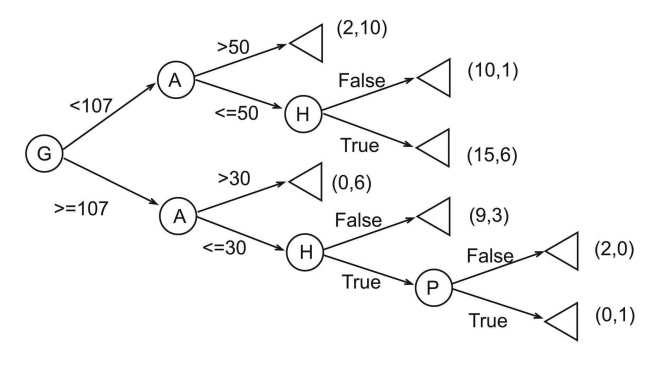
基于Oblivious Tree的决策树,Oblivious有人翻译为对称,有人翻译为遗忘,前者体现了结构上的特点,后者体现了行为上的特点。 从结构上讲,只有一个入度为0的节点且为根节点,所有叶子节点(出度为0)为分类节点,其他节点为中间节点,任意一条从根节点到叶子节点的路径,每个中间节点只出现一次,中间节点,即internal或test node为分类变量,每一层的中间节点变量一样,
注意,每层的每个分类变量一样但判断条件可以不一样 ,所以结构上看是对称的,似乎叫Symmetric Tree更合适。 作者把它称为Oblivious,我认为是基于它行为上的特点,即每个分类变量(中间节点)的触发与整个路径上的所有变量的顺序及它们所处的层次决定,而不是由该变量节点本身决定,所以对比传统决策树,似乎“遗忘”了历史的判断行为,每次都要依着从根节点开始的路径对每个分类变量逐个做判断。典型的结构如下图:
注意看,在age这个属性上,不同的路径可以有不同的判断条件,这种结构在特征选择上比较高效。再一个,每个到达叶子节点的路径上的分类变量都是一样的,这些变量一定是所有输入变量的子集,从这个角度看,其实是在做
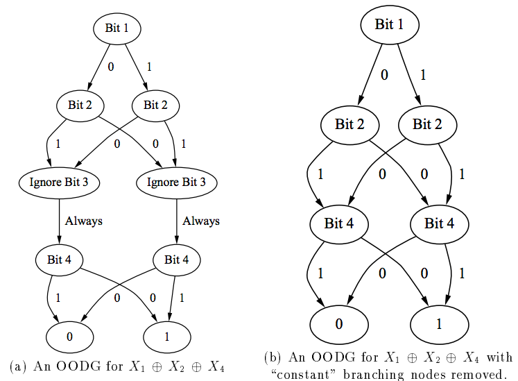
维度缩减 。此外Oblivious Tree也可以看做是Oblivious Oblivious Read-Once Decision Graphs的展开形式,如下图:
详情可以看《Bottom-Up Induction of Oblivious Read-Once Decision Graphs 》一文。
决策表是一种古老但是非常高效的规则匹配方法。用于基于规则的决策系统,如早期的专家系统,匹配模式形如:if A then B ,最典型的有两类:
* Condition-Action Rules
A为条件,B为动作,例如:if x发了工资 then x去银行还月供。
* Logical Rules
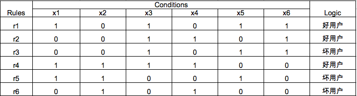
A和B为一阶逻辑表达式,例如:if x是男人 then x是哺乳动物。利用Decision Table可以做分类器,例如最常用的Decision Table Majority,它有两个组成部分:
* Schema,所有决策表中要用到特征的集合。

* Body,依据训练数据得到的命中模式的集合。
典型的例子如下:
回顾Oblivious Decision Trees的结构,非常适合实现一个DTM,定义某个损失函数,构造ODT,最终保留下的中间分类节点集合为Schema,从根节点到叶子节点的所有路径组成的集合是Body。
CatBoost是Yandex在2017年推出的一个GBDT实现框架,论文见:《CatBoost: unbiased boosting with categorical features 》,它的基础学习器是Oblivious Decision Trees,结构上平衡、不容易过拟合、Inference速度极快,支持自动将类别特征处理为数值特征并做特征交叉,为提高模型精度和泛化性能,在Prediction Shift和Gradient Bias上做了理论分析和解决。
1、Prediction Shift
简单回顾第二章Boosting相关内容: \[ \begin{array}{l} F(x)=\sum_{i=1}^Nw_if_i(x)\\ 其中:\\ \quad \quad f_i是第i轮迭代得到的基础分类器\\ \quad \quad w_i是第i个分类器的权重\\ \quad \quad x是样本特征集\\ 定义:\\ \quad \quad \text{(1). 样本总数为 $N$,损失函数定义为$C(F)$,例如: $C(F(x))=\frac{1}{N}\sum_{i=1}^NC(y_iF(x_i))$}\\ \quad \quad \text{(2). $g^t=g^t(x,y)=\frac{\partial C(y,s)}{\partial s}|_{s=F^{t-1}(x)}$,$h^t=h^t(x,y)=\frac{\partial ^2C(y,s)}{\partial s^2}|_{s=F^{t-1}(x)}$}\\ \text{现在我们希望当前轮迭代能够找到一个函数 $f(x)$ ,使得在新分类器$F^t(x)=F^{t-1}(x)+\alpha f(x)$下的损失函数值 $C(F^{t-1}(x)+\alpha f(x))$ 能够下降}\\ 依据泰勒展开式:\\ \because C(F^t(x))=C(F^{t-1}(x)+\alpha f(x))=C(F^{t-1}(x))+\alpha {g^t} f+\frac{1}{2}h^t(\xi)f^2\\ \therefore 根据拉格朗日定理得到:\\ f=-\alpha g^t\\ 由于f是个函数,所以通常用利用最小二乘法对其做拟合:\\ f^t=\mathop{argmin}\limits_{f \in F}~ \mathbb{E}(-f(x)-g^t(x,y))^2 \end{array} \] 这里会有三个问题,即所谓shift,导致最终模型泛化能力下降:
1、训练样本和测试样本梯度值的分布可能不一致;
2、采用类似最小二乘法做函数拟合可能出现偏差,因为背后的假设是梯度值分布服从正态分布,可能与真实世界里的分布不一致;
3、如果每步迭代都使用相同数据集,则得到的模型是有偏的且偏差与数据集大小成反比;反之,如果每步迭代使用相互独立的数据集,则得到的训练模型是无偏的。
以上shift最终造成预测时出现Prediction Shift,假设我们有无限大的标注数据集,那就简单了,每步迭代都独立的抽一个数据集出来,可以训练出无偏模型,但实际上不可能,所以这个问题只可以缓解不能解决,因为你永远不能准确知道真实样本的完美分布,只能摸着石头过河,广告、推荐和搜索里把这个方法叫做E&E(Exploitation & Exploration),本质上Boostng Tree的生成过程就是通过E&E方法迭代生成:使用某个样本集exploit得到当前“最优”的模型,即\(F^{t-1}(x)\) ,用这个模型explore另外一个样本集,根据结果和某种策略优化模型得到新的“最优”模型\(F^t(x)\) ,如此往复,直到找到Exploitation & Exploration的最佳trade-off点。
2、 Ordered boosting
为了缓解Prediction Shift,一个取巧的方法是:
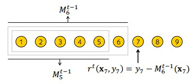
• 用随机排序函数\(\sigma\) 对所有样本重排序
• 维护\(n\) 个独立的模型,每个模型\(M_i\) 由排序后的前\(i\) 个训练样本生成
• 对第\(j\) 个样本的残差用模型\(M_{j-1}\) 来估计
• 原来每个迭代使用由相同样本得到的模型F求梯度的方式改为用辅助模型M估计:
\[g^t:=\frac{\partial L(y,s)}{s}|_{s=F^{t-1}(x)}\Rightarrow g^t:=\frac{\partial L(y,s)}{s}|_{s=M^{t-1}(x)}\] Algorithm 1: Ordered Boosting
input: \(\{(x_k,y_k)\}_{k=1}^n为所有样本,且由\sigma函数重新随机排序, T为树的个数\)
\(M_i \leftarrow 0 \quad for \quad i=1..n,n为模型个数\)
\(for \quad t\leftarrow1 \quad to \quad T \quad do\)
\(\quad for \quad i\leftarrow1 \quad to \quad n \quad do\)
\(\quad \quad for \quad j\leftarrow1 \quad to \quad i \quad do\)
\(\quad \quad \quad\quad g_j\leftarrow\frac{\partial L(y_j,s)}{s}|_{s=M_{j-1}(x_j)}(采用最小二乘损失函数:g_j\leftarrow y_j-M_{j-1}(x_j)\)
\(\quad \quad \Delta M\leftarrow LearnModel(x_j,g_j)\quad for \quad j=1..i\)
\(\quad \quad M_i=M_i+\Delta M\)
\(return \quad M_n\)
由于要训练\(n\) 个模型,时间和空间复杂度都上升了\(n\) 倍,所以这个算法实操性较低。 CatBoost对建树算法做了改进,有对Algorithm 1 算法效率改进的Ordered模式和类似于传统GBDT的Plain模式,其中Ordered模式在小数据集上优势明显。
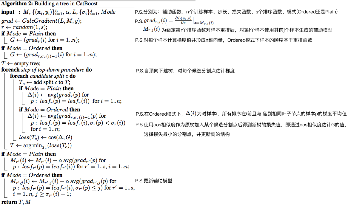
建树的算法Algorithm 2 说明如下:
在Ordered模式下,计算梯度的时间复杂度是\(O(sn^2)\) ,包含选择排序函数的时间、扫描样本生成辅助函数的时间、扫描样本生成梯度的时间,CatBoost在实现时用了几个技巧:
1、不维护全部\(M_{r,j}(i)\) ,转而只维护\(M^{'}_{r,j}(i)=M_{r,2^j}(i),j=1,...,\lceil log_2^n\rceil,\sigma_r(i)\leq2^{j+1}\) ,这样时间复杂度会降到\(O(sn)\)
2、每次迭代时对样本做抽样,这个方法能有效降低过拟合
3、由产生样本过程导致的bias,例如,排第一页的广告比第100页的广告更容易被用户看到、点到,那第100页的广告如果被点击了,这条样本的含金量明显更高,所以位置bias产生的样本可以通过给样本权重的方式或把位置作为特征等方法校正,相关论文可以看:
《Model Ensemble for Click Prediction in Bing Search Ads 》
《Learning to Rank with Selection Bias in Personal Search 》
《PAL: a position-bias aware learning framework for CTR prediction in live recommender systems 》
《The bayesian bootstrap 》
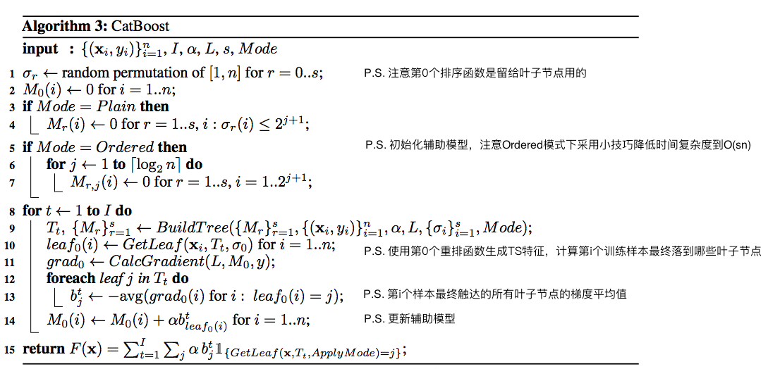
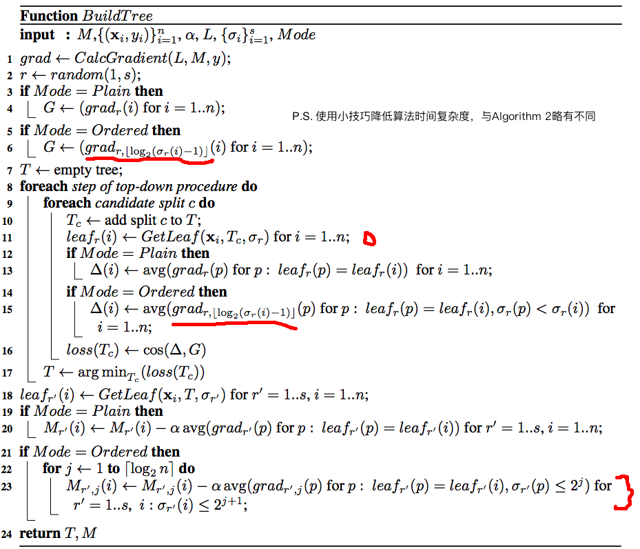
3、完整算法描述
4、代码实践
CatBoost官网上有大量教程,这里给个简单例子:
1、定义Model类
1 2 3 4 5 6 7 8 9 10 11 12 13 14 15 16 17 18 19 20 21 22 23 24 25 26 27 28 29 30 31 32 33 34 35 36 37 38 39 40 41 42 43 44 45 46 47 48 49 50 51 52 53 54 55 56 57 58 59 60 61 62 63 64 65 66 67 68 69 70 71 72 73 74 75 76 77 78 79 80 81 82 83 84 85 86 87 88 89 90 91 92 93 94 95 96 97 98 99 100 101 102 103 104 105 106 107 108 109 110 111 112 113 114 115 116 117 118 """ class CatBoostModel """ import randomfrom sklearn.model_selection import train_test_splitfrom sklearn.preprocessing import LabelEncoderfrom sklearn.model_selection import StratifiedShuffleSplitfrom sklearn.metrics import roc_auc_scoreimport gcimport catboost as cbfrom catboost import *import numpy as npimport pandas as pdclass CatBoostModel (): def __init__ (self, **kwargs ): assert kwargs['catboost_params' ] assert kwargs['eval_ratio' ] assert kwargs['early_stopping_rounds' ] assert kwargs['num_boost_round' ] assert kwargs['cat_features' ] assert kwargs['all_features' ] self.catboost_params = kwargs['catboost_params' ] self.eval_ratio = kwargs['eval_ratio' ] self.early_stopping_rounds = kwargs['early_stopping_rounds' ] self.num_boost_round = kwargs['num_boost_round' ] self.cat_features = kwargs['cat_features' ] self.all_features = kwargs['all_features' ] self.selected_features_ = None self.X = None self.y = None self.model = None def get_selected_features (self, topk ): """ Fit the training data to FeatureSelector Returns ------- list : Return the index of imprtant feature. """ assert topk > 0 self.selected_features_ = self.feature_importance.argsort()[-topk:][::-1 ] return self.selected_features_ def predict (self, X, num_iteration=None ): return self.model.predict(X, num_iteration) def get_fea_importance (self, clf, columns ): importances = clf.feature_importances_ indices = np.argsort(importances)[::-1 ] importance_list = [] for f in range (len (columns)): importance_list.append((columns[indices[f]], importances[indices[f]])) print ("%2d) %-*s %f" % (f + 1 , 30 , columns[indices[f]], importances[indices[f]])) print ("another feature importances with prettified=True\n" ) print (clf.get_feature_importance(prettified=True )) importance_df = pd.DataFrame(importance_list, columns=['Features' , 'Importance' ]) return importance_df def train_test_split (self, X, y, test_size, random_state=2020 ): sss = list (StratifiedShuffleSplit( n_splits=1 , test_size=test_size, random_state=random_state).split(X, y)) X_train = np.take(X, sss[0 ][0 ], axis=0 ) X_eval = np.take(X, sss[0 ][1 ], axis=0 ) y_train = np.take(y, sss[0 ][0 ], axis=0 ) y_eval = np.take(y, sss[0 ][1 ], axis=0 ) return [X_train, X_eval, y_train, y_eval] def catboost_model_train (self, df, finetune=None , target_name='Label' , id_index='Id' ): df = df.loc[df[target_name].isnull() == False ] feature_name = [i for i in df.columns if i not in [target_name, id_index]] for i in feature_name: if i in self.cat_features: if df[i].fillna('na' ).nunique() < 12 : df.loc[:, i] = df.loc[:, i].fillna('na' ).astype('category' ) else : df.loc[:, i] = LabelEncoder().fit_transform(df.loc[:, i].fillna('na' ).astype(str )) if type (df.loc[0 ,i])!=str or type (df.loc[0 ,i])!=int or type (df.loc[0 ,i])!=long: df.loc[:, i] = df.loc[:, i].astype(str ) X_train, X_eval, y_train, y_eval = self.train_test_split(df[feature_name], df[target_name].values, self.eval_ratio, random.seed(41 )) del df gc.collect() catboost_train = Pool(data=X_train, label=y_train, cat_features=self.cat_features, feature_names=self.all_features) catboost_eval = Pool(data=X_eval, label=y_eval, cat_features=self.cat_features, feature_names=self.all_features) self.model = cb.train(params=self.catboost_params, init_model=finetune, pool=catboost_train, num_boost_round=self.num_boost_round, eval_set=catboost_eval, verbose_eval=50 , plot=True , early_stopping_rounds=self.early_stopping_rounds) self.feature_importance = self.get_fea_importance(self.model, self.all_features) metrics = self.model.eval_metrics(data=catboost_eval,metrics=['AUC' ],plot=True ) print ('AUC values:{}' .format (np.array(metrics['AUC' ]))) return self.feature_importance, metrics, self.model
2、定义catboost trainer(里面涉及nni的部分先忽略,后面再讲)
1 2 3 4 5 6 7 8 9 10 11 12 13 14 15 16 17 18 19 20 21 22 23 24 25 26 27 28 29 30 31 32 33 34 35 36 37 38 39 40 41 42 43 44 45 46 47 48 49 50 51 52 53 54 55 56 57 58 59 60 61 62 63 64 65 66 67 68 69 70 71 72 73 74 75 76 77 78 79 80 81 82 83 84 85 86 87 88 89 90 91 92 93 94 95 96 97 98 99 100 101 102 103 104 105 106 107 108 109 110 111 112 113 114 115 116 117 118 119 120 121 122 123 124 125 126 127 128 129 import bz2import urllib.requestimport loggingimport osimport os.pathfrom sklearn.datasets import load_svmlight_filefrom sklearn.preprocessing import LabelEncoderimport nnifrom sklearn.metrics import roc_auc_scoreimport gcimport pandas as pdimport numpy as npfrom model import CatBoostModelfrom catboost.datasets import adultlogger = logging.getLogger('auto_gbdt' ) TARGET_NAME = 'income' def get_default_parameters (): params_cb = { 'boosting_type' : 'Ordered' , 'objective' : 'CrossEntropy' , 'eval_metric' : 'AUC' , 'custom_metric' : ['AUC' , 'Accuracy' ], 'learning_rate' : 0.05 , 'random_seed' : 2020 , 'depth' : 2 , 'l2_leaf_reg' : 3.8 , 'thread_count' : 16 , 'use_best_model' : True , 'verbose' : 0 } return params_cb def get_features_name (): alls = ['age' , 'workclass' , 'fnlwgt' , 'education' , 'education-num' , 'marital-status' , 'occupation' , 'relationship' , 'race' , 'sex' , 'capital-gain' , 'capital-loss' , 'hours-per-week' , 'native-country' ] cats = ['workclass' , 'education' , 'marital-status' , 'occupation' , 'relationship' , 'race' , 'sex' , 'native-country' ] return alls, cats def data_prepare_cleaner (target ): train_df, test_df = adult() le = LabelEncoder() le.fit(train_df[target]) train_df[target] = le.transform(train_df[target]) le.fit(test_df[target]) test_df[target] = le.transform(test_df[target]) return train_df, test_df def cat_fea_cleaner (df, target_name, id_index, cat_features ): df = df.loc[df[target_name].isnull() == False ] feature_name = [i for i in df.columns if i not in [target_name, id_index]] for i in feature_name: if i in cat_features: if df[i].fillna('na' ).nunique() < 12 : df.loc[:, i] = df.loc[:, i].fillna('na' ).astype('category' ) else : df.loc[:, i] = LabelEncoder().fit_transform(df.loc[:, i].fillna('na' ).astype(str )) if type (df.loc[0 ,i])!=str or type (df.loc[0 ,i])!=int or type (df.loc[0 ,i])!=long: df.loc[:, i] = df.loc[:, i].astype(str ) return df def trainer_and_tester_run (train_df, test_df, all_features, cat_features ): RECEIVED_PARAMS = nni.get_next_parameter() logger.debug(RECEIVED_PARAMS) PARAMS = get_default_parameters() PARAMS.update(RECEIVED_PARAMS) logger.debug(PARAMS) cb = CatBoostModel(catboost_params=PARAMS, eval_ratio=0.33 , early_stopping_rounds=20 , cat_features=cat_features, all_features=all_features, num_boost_round=1000 ) logger.debug("The trainning process is starting..." ) train_df = cat_fea_cleaner(train_df, TARGET_NAME, 'index' , cat_features) test_df = cat_fea_cleaner(test_df, TARGET_NAME, 'index' , cat_features) feature_imp, val_score, clf = \ cb.catboost_model_train(df=train_df, target_name=TARGET_NAME, id_index='id' ) logger.info(feature_imp) logger.info(val_score) del train_df gc.collect() logger.debug("The trainning process is ended." ) av_auc = inference(clf, test_df, all_features, cat_features) nni.report_final_result(av_auc) del test_df gc.collect() def inference (clf, test_df, fea, cat_fea ): logger.debug("The testing process is starting..." ) try : y_pred = clf.predict(test_df[fea]) auc = roc_auc_score(test_df[TARGET_NAME].values, y_pred) print ("auc of prediction:{0}" .format (auc)) del test_df gc.collect() logger.debug("The inference process is ended." ) return auc except ValueError: return 0 def run_offline (): alls, cats = get_features_name() print (alls, cats) train_df, test_df = data_prepare_cleaner(TARGET_NAME) print (train_df) print (test_df) trainer_and_tester_run(train_df, test_df, alls, cats) if __name__ == '__main__' : run_offline()
1
2
3
4
5
6
7
8
9
10
11
12
13
14
15
16
17
18
19
20
21
22
23
24
25
26
27
28
29
30
31
32
33
34
35
36
37
38
39
40
41
42
43
44
45
46
47
48
49
50
51
52
53
54
55
56
57
58
59
60
61
62
63
64
65
66
67
68
69
70
71
72
73
74
75
76
77
78
79
80
81
82
83
84
85
86
87
88
89
90
91
92
93
94
95
96
97
98
99
100
101
102
103
104
105
106
107
108
109
110
111
112
113
114
115
116
117
118
119
120
121
122
123
124
125
126
127
128
129
130
131
132
133
134
135
136
137
138
139
140
141
142
143
144
145
146
147
148
149
150
151
152
153
154
155
156
157
158
159
160
161
162
163
164
165
166
167
168
169
170
171
172
173
174
175
176
177
178
179
180
181
182
183
184
185
186
187
188
189
190
191
192
193
194
195
196
197
198
199
200
201
202
203
204
205
206
207
208
209
210
211
212
213
214
215
216
217
218
219
220
221
222
223
224
225
226
227
228
229
230
231
232
233
234
235
236
237
238
239
240
241
242
243
244
245
246
247
248
249
250
251
252
253
254
255
256
257
258
259
260
261
[root@GPU-AI01 cat_test]# python3 catboost_trainer.py ['age', 'workclass', 'fnlwgt', 'education', 'education-num', 'marital-status', 'occupation', 'relationship', 'race', 'sex', 'capital-gain', 'capital-loss', 'hours-per-week', 'native-country'] ['workclass', 'education', 'marital-status', 'occupation', 'relationship', 'race', 'sex', 'native-country'] age workclass fnlwgt education education-num marital-status occupation ... race sex capital-gain capital-loss hours-per-week native-country income 0 39.0 State-gov 77516.0 Bachelors 13.0 Never-married Adm-clerical ... White Male 2174.0 0.0 40.0 United-States 0 1 50.0 Self-emp-not-inc 83311.0 Bachelors 13.0 Married-civ-spouse Exec-managerial ... White Male 0.0 0.0 13.0 United-States 0 2 38.0 Private 215646.0 HS-grad 9.0 Divorced Handlers-cleaners ... White Male 0.0 0.0 40.0 United-States 0 3 53.0 Private 234721.0 11th 7.0 Married-civ-spouse Handlers-cleaners ... Black Male 0.0 0.0 40.0 United-States 0 4 28.0 Private 338409.0 Bachelors 13.0 Married-civ-spouse Prof-specialty ... Black Female 0.0 0.0 40.0 Cuba 0 ... ... ... ... ... ... ... ... ... ... ... ... ... ... ... ... 32556 27.0 Private 257302.0 Assoc-acdm 12.0 Married-civ-spouse Tech-support ... White Female 0.0 0.0 38.0 United-States 0 32557 40.0 Private 154374.0 HS-grad 9.0 Married-civ-spouse Machine-op-inspct ... White Male 0.0 0.0 40.0 United-States 1 32558 58.0 Private 151910.0 HS-grad 9.0 Widowed Adm-clerical ... White Female 0.0 0.0 40.0 United-States 0 32559 22.0 Private 201490.0 HS-grad 9.0 Never-married Adm-clerical ... White Male 0.0 0.0 20.0 United-States 0 32560 52.0 Self-emp-inc 287927.0 HS-grad 9.0 Married-civ-spouse Exec-managerial ... White Female 15024.0 0.0 40.0 United-States 1 [32561 rows x 15 columns] age workclass fnlwgt education education-num marital-status ... sex capital-gain capital-loss hours-per-week native-country income 0 25.0 Private 226802.0 11th 7.0 Never-married ... Male 0.0 0.0 40.0 United-States 0 1 38.0 Private 89814.0 HS-grad 9.0 Married-civ-spouse ... Male 0.0 0.0 50.0 United-States 0 2 28.0 Local-gov 336951.0 Assoc-acdm 12.0 Married-civ-spouse ... Male 0.0 0.0 40.0 United-States 1 3 44.0 Private 160323.0 Some-college 10.0 Married-civ-spouse ... Male 7688.0 0.0 40.0 United-States 1 4 18.0 NaN 103497.0 Some-college 10.0 Never-married ... Female 0.0 0.0 30.0 United-States 0 ... ... ... ... ... ... ... ... ... ... ... ... ... ... 16276 39.0 Private 215419.0 Bachelors 13.0 Divorced ... Female 0.0 0.0 36.0 United-States 0 16277 64.0 NaN 321403.0 HS-grad 9.0 Widowed ... Male 0.0 0.0 40.0 United-States 0 16278 38.0 Private 374983.0 Bachelors 13.0 Married-civ-spouse ... Male 0.0 0.0 50.0 United-States 0 16279 44.0 Private 83891.0 Bachelors 13.0 Divorced ... Male 5455.0 0.0 40.0 United-States 0 16280 35.0 Self-emp-inc 182148.0 Bachelors 13.0 Married-civ-spouse ... Male 0.0 0.0 60.0 United-States 1 [16281 rows x 15 columns] [03/29/2020, 04:36:35 PM] WARNING (nni) Requesting parameter without NNI framework, returning empty dict ['workclass', 'education', 'marital-status', 'occupation', 'relationship', 'race', 'sex', 'native-country'] ['age', 'workclass', 'fnlwgt', 'education', 'education-num', 'marital-status', 'occupation', 'relationship', 'race', 'sex', 'capital-gain', 'capital-loss', 'hours-per-week', 'native-country'] <IPython.core.display.HTML object> MetricVisualizer(layout=Layout(align_self='stretch', height='500px')) 0: test: 0.8316184 best: 0.8316184 (0) total: 79ms remaining: 1m 18s 50: test: 0.9020779 best: 0.9020779 (50) total: 942ms remaining: 17.5s 100: test: 0.9081992 best: 0.9081992 (100) total: 1.71s remaining: 15.2s 150: test: 0.9108707 best: 0.9108707 (150) total: 2.48s remaining: 13.9s 200: test: 0.9133666 best: 0.9133666 (200) total: 3.27s remaining: 13s 250: test: 0.9161119 best: 0.9161119 (250) total: 4.05s remaining: 12.1s 300: test: 0.9181722 best: 0.9181726 (299) total: 4.8s remaining: 11.2s 350: test: 0.9191926 best: 0.9191926 (350) total: 5.56s remaining: 10.3s 400: test: 0.9205207 best: 0.9205207 (400) total: 6.3s remaining: 9.41s 450: test: 0.9210106 best: 0.9210106 (450) total: 7.05s remaining: 8.59s 500: test: 0.9215160 best: 0.9215160 (500) total: 7.81s remaining: 7.78s 550: test: 0.9221193 best: 0.9221193 (550) total: 8.59s remaining: 7s 600: test: 0.9227742 best: 0.9227742 (600) total: 9.37s remaining: 6.22s 650: test: 0.9232136 best: 0.9232136 (650) total: 10.1s remaining: 5.41s 700: test: 0.9234202 best: 0.9234202 (700) total: 10.8s remaining: 4.61s 750: test: 0.9238425 best: 0.9238428 (749) total: 11.6s remaining: 3.83s 800: test: 0.9242466 best: 0.9242466 (800) total: 12.4s remaining: 3.07s 850: test: 0.9244801 best: 0.9244826 (849) total: 13.1s remaining: 2.3s 900: test: 0.9246592 best: 0.9246633 (899) total: 13.8s remaining: 1.52s 950: test: 0.9248365 best: 0.9248397 (949) total: 14.6s remaining: 752ms 999: test: 0.9250032 best: 0.9250045 (998) total: 15.3s remaining: 0us bestTest = 0.9250045138 bestIteration = 998 Shrink model to first 999 iterations. 1) capital-gain 30.102152 2) relationship 21.504190 3) capital-loss 11.414022 4) age 10.377241 5) education-num 7.234561 6) occupation 6.331733 7) hours-per-week 4.476134 8) marital-status 4.354055 9) sex 1.146389 10) education 1.092454 11) workclass 0.776362 12) fnlwgt 0.577348 13) native-country 0.382720 14) race 0.230639 another feature importances with prettified=True Feature Id Importances 0 capital-gain 30.102152 1 relationship 21.504190 2 capital-loss 11.414022 3 age 10.377241 4 education-num 7.234561 5 occupation 6.331733 6 hours-per-week 4.476134 7 marital-status 4.354055 8 sex 1.146389 9 education 1.092454 10 workclass 0.776362 11 fnlwgt 0.577348 12 native-country 0.382720 13 race 0.230639 <IPython.core.display.HTML object> MetricVisualizer(layout=Layout(align_self='stretch', height='500px')) AUC values:[0.83161836 0.85856642 0.85813673 0.86103314 0.86071689 0.86121893 0.86441522 0.86505078 0.8784926 0.87975055 0.88290187 0.88250307 0.88799037 0.8881507 0.89029036 0.88999382 0.88988625 0.89090279 0.89101198 0.89160979 0.89201995 0.89295319 0.89335747 0.89347394 0.89391874 0.89388563 0.89537425 0.89577286 0.89558464 0.89714728 0.89720971 0.89743348 0.89766614 0.89780103 0.89835231 0.89859723 0.89845935 0.89914869 0.89911805 0.89974913 0.89990595 0.90033138 0.90038467 0.90098889 0.90072697 0.90107988 0.90084311 0.90124622 0.90129837 0.90169675 0.90207794 0.90213554 0.90252241 0.90278218 0.90291333 0.90347889 0.90362643 0.90369515 0.90384743 0.90364836 0.90427544 0.90441459 0.90463238 0.90473693 0.90474323 0.9047752 0.90479827 0.90473968 0.90509671 0.9052363 0.90524989 0.90552186 0.90563292 0.90562407 0.90597002 0.90596054 0.90612973 0.90613532 0.90626529 0.90624885 0.90629925 0.9065094 0.90687207 0.90713255 0.90713464 0.90714229 0.90716147 0.90720291 0.90736582 0.9074965 0.90754282 0.90756655 0.907661 0.90770332 0.9077639 0.90790968 0.9079417 0.90798504 0.90802753 0.90811397 0.90819922 0.90826913 0.90827529 0.90832273 0.90834522 0.90836268 0.90852687 0.90865518 0.90867734 0.90877048 0.9088641 0.90892809 0.90899198 0.90898232 0.90901235 0.90917898 0.90931463 0.90933462 0.90946639 0.90955688 0.90957899 0.90955768 0.9096148 0.90963834 0.90960947 0.9097182 0.90968601 0.90968109 0.90973949 0.90986055 0.90987831 0.90990626 0.90988658 0.90996061 0.9100206 0.91016861 0.9102051 0.91031329 0.91035212 0.91039234 0.91038859 0.91055811 0.91059551 0.91060905 0.91068851 0.91069095 0.91070089 0.91075133 0.9107646 0.91083661 0.91087072 0.91088294 0.91089601 0.9109779 0.91109368 0.91112637 0.91117719 0.91131483 0.91133695 0.91135528 0.91138891 0.91139388 0.91141477 0.91143149 0.91147063 0.91155253 0.91162016 0.91166083 0.91172069 0.91181031 0.91196481 0.91200488 0.91207325 0.91211531 0.91215074 0.91216651 0.91216438 0.91216644 0.91217042 0.91222321 0.91224604 0.91226224 0.91238903 0.91245311 0.91250443 0.9125005 0.91256733 0.9126408 0.91267537 0.9127926 0.91283471 0.91296865 0.91309914 0.91321599 0.9132311 0.91326122 0.91331664 0.9133272 0.91333757 0.91335631 0.91336663 0.91339323 0.91351306 0.91353504 0.91364762 0.91371905 0.91374356 0.91382455 0.91383544 0.91387963 0.9138874 0.9139162 0.9139656 0.91401361 0.91409119 0.91417138 0.91415125 0.91426151 0.91427733 0.91430731 0.91443747 0.91448261 0.91453059 0.91459567 0.91462631 0.91465691 0.91466103 0.91475955 0.91475329 0.91484831 0.91488644 0.9149258 0.91522573 0.91525917 0.91535504 0.91542878 0.91546454 0.91549223 0.91553097 0.91555825 0.91559304 0.91562558 0.91568611 0.91569478 0.91571794 0.9157357 0.91576043 0.91577251 0.9158588 0.91609757 0.91611192 0.91617368 0.91615905 0.91616662 0.91621344 0.91624148 0.91624617 0.916279 0.91631196 0.91642947 0.91647835 0.91652667 0.91651392 0.91652581 0.91653713 0.91655006 0.91665427 0.91667051 0.916788 0.91681452 0.91685526 0.91696372 0.91706001 0.91709748 0.91709928 0.91717672 0.91719126 0.91729565 0.91739161 0.91742034 0.9174929 0.91750469 0.91754306 0.9175746 0.91757541 0.91759738 0.91761036 0.91759407 0.91763139 0.91772489 0.91776103 0.9179556 0.9179898 0.91801864 0.91801737 0.91803603 0.91805739 0.91813814 0.91814534 0.91817263 0.9181722 0.91824609 0.91827275 0.91829577 0.91829899 0.91831358 0.91837373 0.91842195 0.91842025 0.91844374 0.91845804 0.91856584 0.91857612 0.91863774 0.91862941 0.91863533 0.91871476 0.91873683 0.91873685 0.91873453 0.91876589 0.91877062 0.91877522 0.91875817 0.91876122 0.9187661 0.91875142 0.91882763 0.91882948 0.91885122 0.91885425 0.91883814 0.91885245 0.91885491 0.91889654 0.91892941 0.91899658 0.91898947 0.91903944 0.91905251 0.91906383 0.91905976 0.91905803 0.91906125 0.91911411 0.91912297 0.91911189 0.9191422 0.91916427 0.91918881 0.91919262 0.9192038 0.91922066 0.91922383 0.91924121 0.91924974 0.91929625 0.91931439 0.9193681 0.91936356 0.9194005 0.91940401 0.91942551 0.91941168 0.91949196 0.91950447 0.91950522 0.91950731 0.91951408 0.91954548 0.919564 0.91956135 0.91961966 0.91962117 0.91961662 0.91963093 0.91963782 0.9197918 0.91981146 0.91984902 0.91987796 0.91986474 0.91986896 0.91988572 0.91999293 0.91999407 0.9200143 0.92006417 0.920051 0.92006654 0.92015715 0.92027774 0.92028039 0.92028351 0.92029304 0.9203403 0.92041614 0.9204284 0.920495 0.92051366 0.92052067 0.92052967 0.92054984 0.92056874 0.92059948 0.9206144 0.92060015 0.92060062 0.9206 0.92060142 0.92060772 0.92063425 0.92063752 0.92064007 0.92064424 0.92065741 0.92066167 0.92067399 0.92068185 0.92068403 0.92072576 0.92073774 0.92074077 0.92074873 0.92073982 0.92076398 0.92077724 0.92078624 0.92078373 0.92078809 0.92077483 0.92077691 0.92080732 0.92081864 0.92082224 0.92081307 0.92081577 0.92081407 0.9208495 0.92085911 0.92088312 0.92088725 0.92088677 0.92088559 0.92089568 0.92089648 0.92090354 0.92092367 0.92092732 0.92094607 0.92101058 0.92102503 0.92103919 0.92102465 0.92103474 0.92103725 0.92102598 0.92102195 0.92102607 0.92103857 0.92103682 0.92103957 0.92106103 0.92107088 0.92107722 0.92108452 0.92108708 0.92114306 0.92115324 0.92119644 0.9212017 0.92121074 0.92122964 0.92124253 0.92124826 0.92127222 0.92129136 0.92131528 0.92131712 0.92132233 0.9213274 0.92132897 0.92131902 0.92132323 0.92133725 0.92138855 0.92138997 0.92144297 0.92145268 0.92144453 0.92144766 0.92148863 0.92148243 0.92148764 0.92149299 0.92150881 0.92149493 0.92149905 0.92150045 0.92151196 0.92151603 0.92152768 0.92153251 0.92151722 0.92152228 0.92152569 0.92153124 0.92162734 0.92162582 0.92164117 0.9216549 0.92165462 0.92171068 0.92171977 0.92172706 0.92172754 0.92173966 0.92175084 0.92175719 0.92175633 0.92175221 0.92176424 0.92176529 0.92177016 0.92177178 0.92178025 0.92176628 0.92184211 0.9218522 0.92185713 0.92185623 0.92186669 0.92191529 0.92194717 0.92195285 0.92197383 0.92197056 0.92197052 0.92197658 0.92198013 0.92196483 0.92197075 0.92197885 0.92198245 0.92199188 0.92204175 0.92204227 0.92209778 0.92210214 0.92210863 0.92211934 0.92216049 0.92216462 0.92216983 0.92217963 0.92217537 0.92221117 0.92241212 0.92241638 0.92242576 0.92243073 0.92243177 0.92244111 0.92245001 0.92246045 0.9224605 0.92249186 0.92249266 0.9225063 0.92253676 0.92254249 0.92254519 0.92255234 0.92255675 0.9225657 0.92257275 0.92256906 0.92257072 0.92255637 0.92255892 0.922562 0.92256087 0.92257162 0.92257129 0.92257129 0.92257015 0.92255466 0.92255267 0.92254007 0.92253922 0.92254197 0.92254647 0.92254566 0.9225891 0.9225908 0.92258696 0.92259497 0.92259644 0.92275269 0.9227705 0.92277424 0.92276742 0.92277045 0.92277491 0.92278784 0.92278968 0.9227921 0.92279944 0.92280498 0.92281464 0.92282772 0.92282279 0.92295612 0.92295963 0.92295584 0.92297024 0.92295882 0.92296086 0.92295636 0.92296015 0.92296214 0.92297611 0.92297597 0.92297367 0.92297282 0.9229821 0.92299015 0.92299285 0.92299162 0.92299494 0.92304206 0.92307967 0.92308431 0.92310553 0.92310695 0.92310871 0.92310894 0.9231188 0.92311927 0.92312131 0.92313343 0.92313457 0.92313679 0.92313154 0.92313566 0.92314866 0.92315825 0.92315967 0.92320145 0.92320557 0.92321357 0.92322352 0.92323133 0.92323763 0.92323815 0.92324663 0.92324834 0.92325137 0.92325492 0.92325402 0.92325374 0.92326515 0.92327003 0.92327538 0.92326444 0.92326927 0.92326937 0.92325672 0.92327946 0.92327837 0.92327979 0.92328097 0.92328386 0.92329125 0.92329248 0.92329977 0.92330783 0.92330854 0.92331124 0.92331299 0.92334018 0.92333804 0.92333752 0.92334894 0.92334851 0.92334979 0.92335064 0.92335164 0.92336736 0.92336869 0.92337068 0.9233623 0.92336433 0.92336395 0.92336964 0.92337428 0.92338446 0.92339521 0.92339592 0.92340004 0.92342017 0.92341999 0.92342126 0.92342264 0.92341984 0.92341984 0.92341833 0.92340795 0.92341307 0.92342212 0.92346853 0.92346801 0.92349373 0.92351225 0.92351931 0.92352476 0.92356085 0.92356151 0.92356483 0.92357894 0.92361887 0.92361683 0.92362503 0.92362484 0.92364317 0.92366462 0.92366391 0.92366415 0.92366709 0.92367481 0.92368707 0.92368769 0.92368816 0.92368991 0.92368925 0.92369735 0.92372847 0.92372814 0.92372667 0.92373089 0.92373169 0.92373538 0.92376077 0.92376134 0.92377977 0.9238052 0.92380307 0.92382703 0.92383556 0.92384276 0.92384248 0.92384338 0.92384195 0.92384991 0.92384778 0.92385673 0.92385702 0.92385579 0.92388179 0.92390358 0.92390452 0.92392219 0.92393938 0.9239624 0.92396657 0.92397055 0.92397022 0.92398855 0.92398784 0.92399916 0.92401161 0.92402559 0.92402535 0.92412785 0.92413405 0.92415006 0.92416323 0.92416356 0.92416346 0.9241593 0.92415797 0.92415541 0.92415636 0.92415508 0.92415357 0.9241574 0.92417905 0.92419297 0.92420628 0.92421429 0.92421362 0.92421457 0.92422599 0.92422475 0.92422423 0.92422291 0.92422414 0.9242293 0.92423915 0.92424469 0.92424659 0.92424834 0.9242482 0.92426392 0.92426804 0.9242796 0.92428093 0.92429978 0.92430196 0.92430196 0.92432313 0.92432455 0.9243191 0.92431726 0.9243156 0.9243146 0.92432185 0.924339 0.92433824 0.92435922 0.92436339 0.92436391 0.92437964 0.92437731 0.92438267 0.92438025 0.92437954 0.92437973 0.92441307 0.92441795 0.92441701 0.92442023 0.9244314 0.92442975 0.92442918 0.92442804 0.92442899 0.92443202 0.92443264 0.92443145 0.92444026 0.92445457 0.92445348 0.92445267 0.92445163 0.92445144 0.92446295 0.92447209 0.92446982 0.92448261 0.92448014 0.92448966 0.92450439 0.92450236 0.92450188 0.92450184 0.92449956 0.92451074 0.92451017 0.9245222 0.92452661 0.92452457 0.92453395 0.92453172 0.92454541 0.92454967 0.92454584 0.92454304 0.92454058 0.92454039 0.92453722 0.92455214 0.92455304 0.92454953 0.92456061 0.92457629 0.9245798 0.92457681 0.92459439 0.92460656 0.92462025 0.92461693 0.92462337 0.92461906 0.92463341 0.9246309 0.92463697 0.92463474 0.92463332 0.92463242 0.92462896 0.92462574 0.92463891 0.92464047 0.92464241 0.92464023 0.92464147 0.92465189 0.92465809 0.9246633 0.92465923 0.92466605 0.92466898 0.92467012 0.92466695 0.92466572 0.92467879 0.92468964 0.92471355 0.92472397 0.92472525 0.9247262 0.92473302 0.92472966 0.92473449 0.92473468 0.92473392 0.92473316 0.92473132 0.92472805 0.92472582 0.92472492 0.92472293 0.9247263 0.92473454 0.92473511 0.92473743 0.92473648 0.92475415 0.92476172 0.92475898 0.92477077 0.92479057 0.92479355 0.92479284 0.92480303 0.9248143 0.92481302 0.92482448 0.92482211 0.92482301 0.92482368 0.92482808 0.92482638 0.92482931 0.92483178 0.92483741 0.92483784 0.9248386 0.92483969 0.92483646 0.9248404 0.92485238 0.92485067 0.92486796 0.92488321 0.92488009 0.92487786 0.92487805 0.92488516 0.92488994 0.92489098 0.92490003 0.92490704 0.92490391 0.92491362 0.92492802 0.92493299 0.9249463 0.92494289 0.92493906 0.92493816 0.92494223 0.92493996 0.9249382 0.92493849 0.9249491 0.92494697 0.92494711 0.92495838 0.92495838 0.92497013 0.92498078 0.92497794 0.92497695 0.92497827 0.92497619 0.924976 0.92498211 0.92498495 0.92499078 0.92500338 0.92500087 0.92500049 0.92499874 0.92499874 0.92499883 0.92499935 0.92500451] AUC of prediction:0.8603217542453206
2.6 人工神经网络-Neural Network 神经网络在维基百科上的定义是:NN is a network inspired by biological neural networks (the central nervous systems of animals, in particular the brain) which are used to estimate or approximate functions that can depend on a large number of inputs that are generally unknown.(from wikipedia)
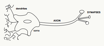
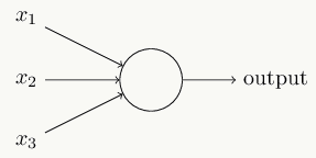
2.6.1 神经元 神经元是神经网络和SVM这类模型的基础模型和来源,它是一个具有如下结构的线性模型:
其输出模式为:
\[ \begin{array}{l} output & = & \left\{ \begin{array}{1} 0 & if~ \sum_j w_j x_j + b \leq 0 \\ 1 & if~ \sum_j w_j x_j + b> 0 \end{array} \right. \end{array} \]
示意图如下:
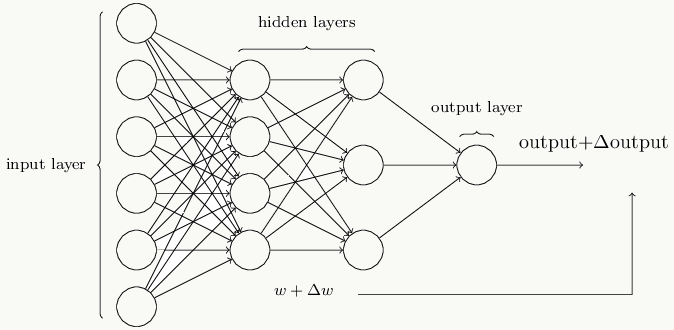
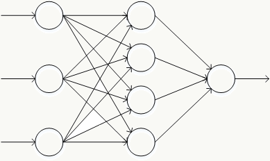
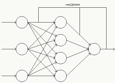
2.6.2 神经网络的常用结构 神经网络由一系列神经元组成,典型的神经网络结构如下:
其中最左边是输入层,包含若干输入神经元,最右边是输出层,包含若干输出神经元,介于输入层和输出层的所有层都叫隐藏层,由于神经元的作用,任何权重的微小变化都会导致输出的微小变化,即这种变化是平滑的。
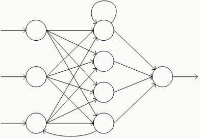
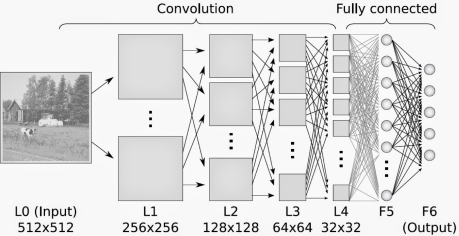
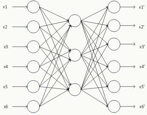
神经元的各种组合方式得到性质不一的神经网络结构 :
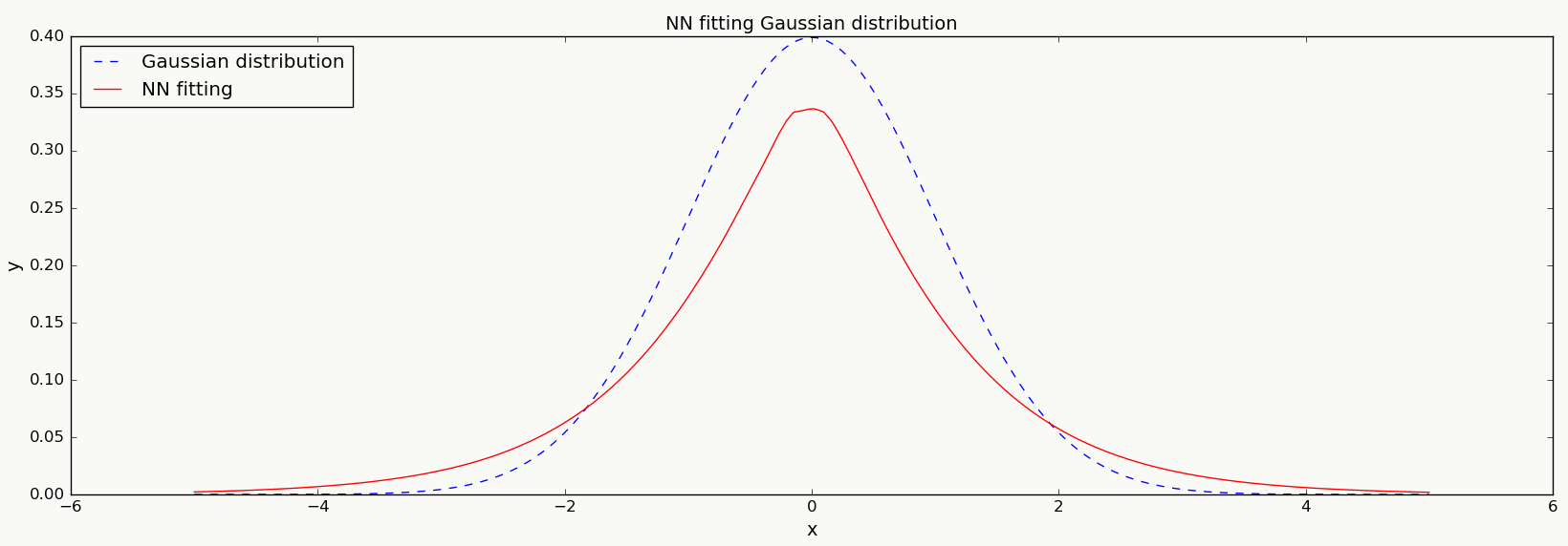
前馈神经网络 反向传播神经网络 循环神经网络 卷积神经网络 自编码器 Google DeepMind 记忆神经网络(用于AlphaGo) 2.6.3 一个简单的神经网络例子 假设随机变量 \(x \sim N(0,1)\) , 使用3层神经网络拟合该分布:
1
2
3
4
5
6
7
8
9
10
11
12
13
14
15
16
17
18
19
20
21
22
23
24
25
26
27
28
29
30
31
32
33
34
35
36
37
38
39
40
41
42
43
44
45
46
47
48
49
50
51
52
53
54
55
56
57
58
59
60
61
62
import numpy as np import matplotlib matplotlib.use('Agg') import matplotlib.pyplot as plt import random import math import keras from keras.models import Sequential from keras.layers.core import Dense,Dropout,Activation def gd(x,m,s): left=1/(math.sqrt(2*math.pi)*s) right=math.exp(-math.pow(x-m,2)/(2*math.pow(s,2))) return left*right def pt(x, y1, y2): if len(x) != len(y1) or len(x) != len(y2): print 'input error.' return plt.figure(num=1, figsize=(20, 6)) plt.title('NN fitting Gaussian distribution', size=14) plt.xlabel('x', size=14) plt.ylabel('y', size=14) plt.plot(x, y1, color='b', linestyle='--', label='Gaussian distribution') plt.plot(x, y2, color='r', linestyle='-', label='NN fitting') plt.legend(loc='upper left') plt.savefig('ann.png', format='png') def ann(train_d, train_l, prd_d): if len(train_d) == 0 or len(train_d) != len(train_l): print 'training data error.' return model = Sequential() model.add(Dense(30, input_dim=1)) model.add(Activation('relu')) model.add(Dense(30)) model.add(Activation('relu')) model.add(Dense(1, activation='sigmoid')) model.compile(loss='mse', optimizer='rmsprop', metrics=['accuracy']) model.fit(train_d,train_l,batch_size=250, nb_epoch=50, validation_split=0.2) p = model.predict(prd_d,batch_size=250) return p if __name__ == '__main__': x = np.linspace(-5, 5, 10000) idx = random.sample(x, 900) train_d = [] train_l = [] for i in idx: train_d.append(x[i]) train_l.append(gd(x[i],0,1)) y1 = [] y2 = [] for i in x: y1.append(gd(i,0,1)) y2 = ann(np.array(train_d).reshape(len(train_d), 1), np.array(train_l), np.array(x).reshape(len(x), 1)) pt(x, y1, y2.tolist())
 本章对方差和偏差、损失函数、常用的机器学习模型(包括:线性回归、支持向量机、逻辑回归、GBDT、CatBoost、RF)等做了回顾。