 本章对机器视觉方面的深度神经网络做了历史回顾及原理介绍,由于这方面技术发展很快,所以文章内容主要集中于几个极具代表性的框架。
5. 深度神经网络
深度学习是基于多层神经网络的一种对数据进行自动表征学习的框架,能使人逐步摆脱传统的人工特征提取过程,它的基础之一是distributed representation,读论文时注意以下概念区分:
Distributional representation
Distributional representation是基于某种分布假设和上下文共现的一类表示方法,比如,对于词的表示来说:有相似意义的词具有相似的分布。
从技术上讲这类方法的缺点是:通常对存储敏感,在representation上也不高效,但是优点是:算法相对简单,甚至像LSA那样简单的线性分解就行。
几类常见的Distributional representation模型:
Distributed representation
Distributed representation是对实体(比如:词、车系编号、微博用户id等等)稠密、低维、实数的向量表示,也就是常说的embedding,它不需要做分布假设,向量的每个维度代表实体在某个空间下的隐含特征。
从技术上讲它的缺点是:计算代价较高,算法往往不简单直接,通常通过神经网络/深度神经网络实现,优点是:对原始信息的有效稠密压缩表示,不仅仅是考虑“共现”,还会考虑其他信息,比如:“时序”等。
几类常见的Distributed representation模型:
Collobert and Weston embeddings
HLBL embeddings
关于Distributional representation和Distributed representation以及几个相关概念,看论文Word representations: A simple and general method for semi-supervised learning即可明了。
5.1 反向传播
反向传播是神经网络参数学习的必备工具,以经典的多层前向神经网络为例: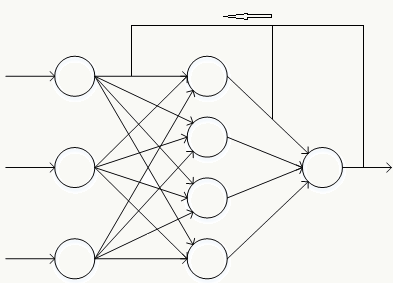
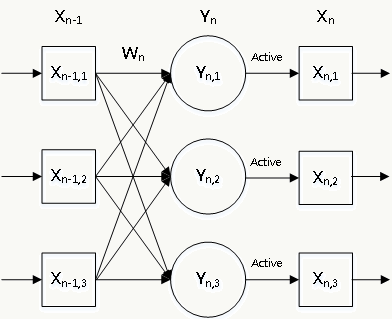
假设:
1、当\(n=o\)为输出层时,整个网络的误差表示为:\(E^o(X^o,D)\),其中\(D\)为期望输出;
2、任意层的激活函数表示为\(F(x)\);
3、第\(n\)层输入为上一层输出\(X^{n-1}\),该层权重为\(W^n\),则:
该层中间输出为:\(Y^n=W^nX^{n-1}\) 该层输出为:\(X^n=F(Y^n)\)。
那么误差反向传播原理为:
\[ \begin{array}{l} \frac{\partial E^o}{\partial Y^n}=F'(Y^n)\frac{\partial E^o}{\partial X^n}\\ \frac{\partial E^o}{\partial W^n}=X^{n-1}\frac{\partial E^o}{\partial Y^n}\\ \frac{\partial E^o}{\partial X^{n-1}}=(W^n)^T\frac{\partial E^o}{\partial Y^n}\\ \end{array} \] 其中,定义\(\delta^n=\frac{\partial E^o}{\partial Y^n}\)为误差反向传播时第\(n\)层某个节点的“误差敏感度”。
参数学习过程为:\(W_t=W_{t-1}-\eta \frac{\partial E}{\partial W_{t-1}}\),其中\(\eta\)的讨论前文已经做过不在赘述,应用导数的链式传导原理,所有层的权重都将得到更新。
5.2 卷积网络结构演化史
网络结构的发展历程更像是一个实验科学的过程,人们通过不断地尝试和实验来得到与验证各种网络结构。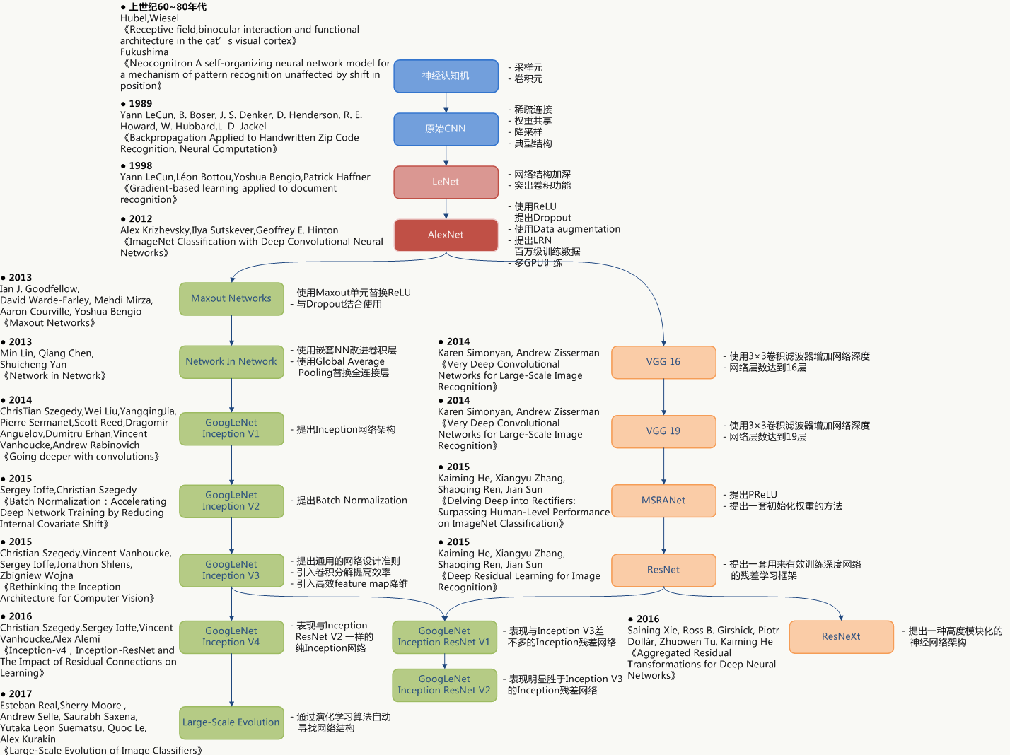
5.3 CNN基本原理
卷积神经网络是我认为非常好用的一类神经网络结构,当数据具有局部相关性时是一种比较好选择,在图像、自然语言处理、棋类竞技、新药配方研制等方面有广泛应用。比如,经典的LeNet-5网络结构:5.3.1 Sigmoid激活函数
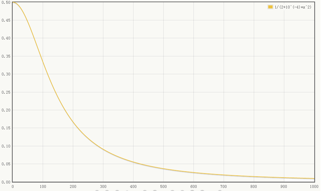
激活函数是神经网络必备工具,而Sigmoid激活函数是早期神经网络最普遍的选择。Sigmoid函数是类神奇的函数,广义上所有形为“S”的函数都可叫做Sigmoid函数,从早期的感知机模型中Sigmoid函数就被用来模拟生物细胞的激活反应,所以又被叫做激活函数,从数学角度看,Sigmoid函数对中间信号增益较大而对两侧信号增益小,所以在信号的特征空间映射上效果好。 从生物角度看,中间部分类似神经元的兴奋状态而两侧类似神经元的抑制状态,所以神经网络在学习时,区分度大的重要特征被推向中间而次要特征被推向两侧。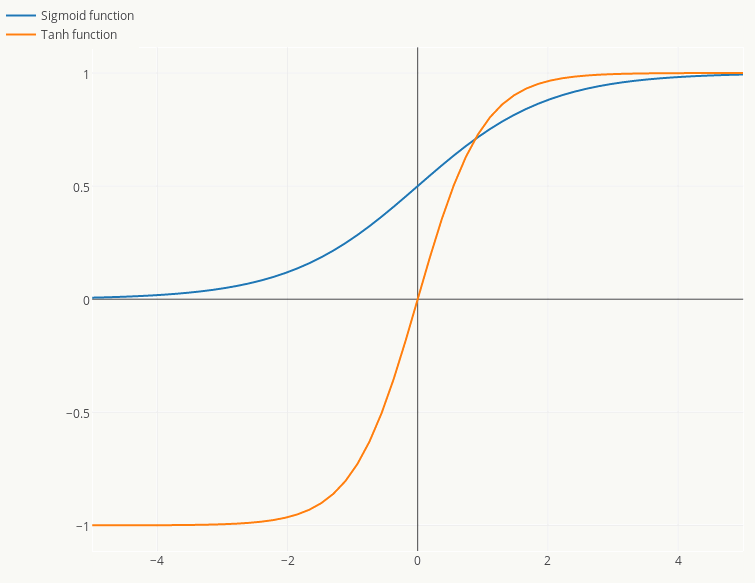
\[ logistic(x)=\frac{1}{1+e^{-x}}\\ tanh(x)=2logistic(2x)-1 \]
Logistic函数最早是Pierre François Verhulst在研究人口增长问题时提出的,由于其强悍的普适性(从概率角度的理解见前面对Logistic Regression的讲解)而被广泛应用(在传统机器学习中派生出Logistic Regression),但是实践中,它作为激活函数有两个重要缺点:
梯度消失问题(Vanishing Gradient Problem)
从前面BP的推导过程可以看出:误差从输出层反向传播时,在各层都要乘以当前层的误差敏感度,而误差敏感度又与\(Sigmoid'(x)\)有关系,由于\(Sigmoid'(x)\in(0,1)\) 且\(x\in(0,1) \text{ or }x\in(-1,1)\),可见误差会从输出层开始呈指数衰减,这样即使是一个4层神经网络可能在靠近输入层的部分都已经无法学习了,更别说“更深”的网络结构了,Hinton提出的逐层贪心预训练方法在一定程度缓解了这个问题但没有真正解决。
激活输出非0均值问题
假设一个样本一个样本的学习,当前层输出非0均值信号给下一层神经元时:如果输入值大于0,则后续通过权重计算出的梯度也大于0,反之亦然,这会导致整个网络训练速度变慢,虽然采用batch的方式训练会缓解这个问题,但毕竟在训练中是拖后腿的,所以Yann LeCun在《Efficient BackPro》一文中也提到了解决的trick。
Tanh函数是另外一种Sigmoid函数,它的输出是0均值的,Yann LeCun给出的一种经验激活函数形式为:\[f(x)=1.7159 \cdot tanh(\frac{2}{3}x)\]但这个函数依然解决不了梯度消失问题,后续介绍其他网络结构时会看到在激活函数层面上的演化。
CNN的典型特点是:局部相关性(稀疏连接)、权重与偏置共享及采样,一套典型的结构由输入层、卷积层、采样层、全连接层、输出层组成。
5.3.2 输入层
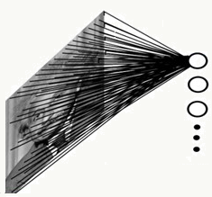
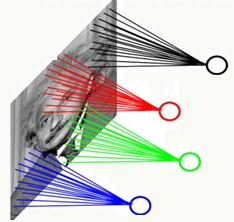
CNN的输入层一般为一个n维矩阵,可以是图像、向量化后的文本等等。比如一幅彩色图像: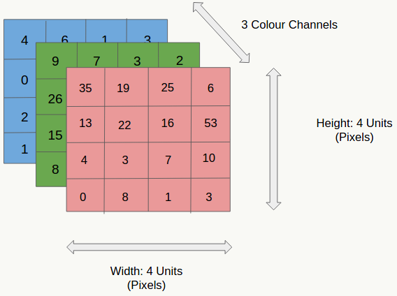
5.3.3 卷积层
卷积操作在数学上的定义如下: \[f*g = \int^{\infty}_{-\infty}(\sum^{\infty}_{-\infty}) f(\tau)g(x-\tau)d\tau \tag{1}\]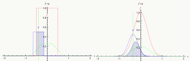
但对于我们正在讲的CNN中的卷积并不是严格意义的卷积(Convolution)操作,而是变体Cross-Correlation: \[f★ g = \int^{\infty}_{-\infty}(\sum^{\infty}_{-\infty}) \bar{f}(\tau)g(x+\tau)d\tau \tag{1}\] 其中\(\bar{f}\)为\(f\)的Complex Conjugate。
卷积层的作用:
当数据及其周边有局部关联性时可以起到滤波、去噪、找特征的作用;
每一个卷积核做特征提取得到结果称为feature map,利用不同卷积核做卷积会得到一系列feature map,这些feature map大小为长×宽×深度(卷积核的个数)并作为下一层的输入。
以图像处理为例,卷积可以有至少3种理解:
平滑
当设置一个平滑窗口后(如3×3),除了边缘外,图像中每个像素点都是以某个点为中心的窗口中各个像素点的加权平均值,这样由于每个点都考虑了周围若干点的特征,所以本质上它是对像素点的平滑。
滤波
将信号中特定波段频率过滤的操作,是防干扰的一类方法,如果滤波模板(卷积核)是均匀分布,那么滤波就是等权滑动平均,如果模板是高斯分布,那么滤波就是权重分布为钟形的加权滑动平均,不同的模板能得到图像的不同滤波后特征。
投影
卷积是个内积操作,如果把模板(卷积核)拉直后看做一个基向量,那么滑动窗口每滑动一次就会产生一个向量,把这个向量往基向量上做投影就得到feature map,如果模板有多个,则组成一组基,投影后得到一组feature map。
卷积和权重共享可以在保证效果的基础上大大降低模型复杂度,说明如下:
输入层为5×5矩阵,卷积核为3×3矩阵,隐藏层为:3×3矩阵: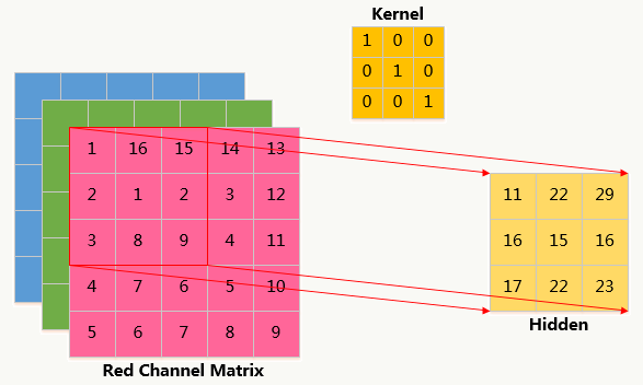
采用全连接神经网络
参数个数为:5×5×9=225
![]()
采用局部连接神经网络
隐藏层只与3×3大小的局部像素相连,参数个数为:3×3×9=81
![]()
采用局部连接权重共享神经网络
所有隐藏层共享权值,且权值为卷积核,参数个数为:3×3×1=9,共享权重的本质含义是对图片某种统计模式的描述,这种模式与图像位置无关。
![]()
5.3.4 Zero-Padding
Zero-Padding是一种影响输出层构建的方法,思路比较简单:把输入层边界外围用0填充,当我们希望输出空间维度和输入空间维度大小一样时可以用此方法,例如下图:当输入为4×4,卷积核为3×3时,利用Zero-Padding可以让输出矩阵也是4×4。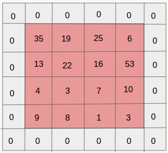
Zero-Padding一方面让你的网络结构设计更灵活,一方面还可以保留边界信息,不至于随着卷积的过程信息衰减的太快。 大家如果使用Tenserflow会知道它的padding参数有两个值:SAME,代表做类似上图的Zero padding,使得输入的feature map和输出的feature map有相同的大小;VALID,代表不做padding操作。
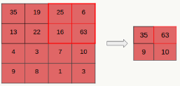
5.3.5 采样层(pooling)
通过卷积后。模型的参数规模大幅下降,但对于复杂网络参数个数依然很多,且容易造成过拟合,所以一种自然的方式就是做下采样,采样依然采用滑动窗口方式,常用采样有Max-Pooling(将Pooling窗口中的最大值作为采样值)和Mean-Pooling(将Pooling窗口中的所有值相加取平均,用平均值作为采样值),一个例子如下: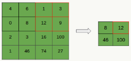
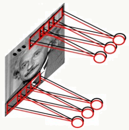
另外,如果卷积层的下一层是pooling层,那么每个feature map都会做pooling,与人类行为相比,pooling可以看做是观察图像某个特征区域是否有某种特性,对这个区域而言不关心这个特性具体表现在哪个位置(比如:看一个人脸上某个局部区域是否有个痘痘)。
5.3.6 全连接样层
全连接层一般是CNN的最后一层,它是输出层和前面若干层的过渡层,用来组织生成特定节点数的输出层。
5.3.7 参数求解
对于多分类任务,假设损失函数采用平方误差: \[E(x)=\sum_{i=0}^N\sum_{k=0}^C(t^k_i-y^k_i)^2\],\(C\)为分类个数,\(N\)为样本数。 下面以一个样本为例推导CNN的原理: \[E(x)=\sum_{k=0}^C(t^k-y^k)^2\]
全连接层
为方便,假设偏置项\(b\)都被放入权重项\(W\)中,则对全连接层来说第\(n\)层与第\(n-1\)层的关系为: \[ \begin{array}{l} X^n=F(Y^n)\\ Y^n=W^nX^{n-1} \end{array} \] 反向传播定义为:
\(\because\) \[ \begin{array}{l} \delta^n=\frac{\partial E}{\partial Y^n}=F'(Y^n)\frac{\partial E}{\partial X^n}\\ \frac{\partial E}{\partial W^n}=X^{n-1}(\delta^n)^T\\ \frac{\partial E}{\partial X^{n-1}}=(W^n)^T\frac{\partial E^o}{\partial Y^n}\\ \end{array} \] \(\therefore\) \[ \left\{ \begin{aligned} \delta^n = & F'(Y^n)(W^{n+1})^T\delta^{n+1} \\ \delta^L = & F'(Y^L)(t^{n}-y^n) \quad\text{L表示最后一层}\\ \frac{\partial E}{\partial W^n} = & X^{n-1}(\delta^n)^T \end{aligned} \right. \] \[ \begin{array}{l} \Delta W^n=-\eta \frac{\partial E}{\partial W^n}\\ W^n=W^{n-1}+\Delta W^n \end{array} \]
卷积层 由于卷积操作、共享权重的存在,这一中间层的输出会被定义为: \[ \begin{array}{l} X_j^n=F(Y_j^n)\\ Y_j^n=\sum_{i\in M_j}X_i^{n-1}k_{ij}^n+b_j^n \end{array} \] 其中:\(n\)为当前卷积层,\(j\)为卷积层某个特征,\(k\)为卷积核,\(b\)为偏置。
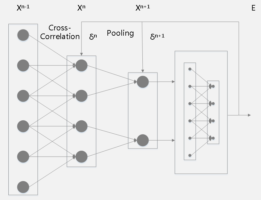
1、当前层为卷积层且下一层为下采样层(pooling)时,反向传播的原理为:
\(\delta^n_j = \beta_j^{n+1}(F'(Y^n)upsampled(\delta^{n+1}_j))\)
下面解释\(upsampled\)和\(\beta\)操作:
卷积层在卷积窗口内的像素与下采样层的像素是多对一的关系,即下采样层的一个神经元节点对应的误差灵敏度对应于上一层卷积层的采样窗口大小的一块像素,下采样层每个节点的误差敏感值由上一层卷积层中采样窗口中节点的误差敏感值联合生成,因此,为了使下采样层的误差敏感度窗口大小和卷积层窗口(卷积核)大小一致,就需要对下采样层的误差敏感度做上采样\(upsampled\)操作,相当于是某种逆映射操作,对于max-pooling、mean-polling或者各自的加权版本来说处理方法类似:
![]()
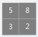
\[ \begin{array}{l} \delta^n_j=F'(Y^n_j)\frac{\partial E}{\partial X^n_j}\\ \frac{\partial E}{\partial X^{n}_j}=(W^{n+1}_j)^T\frac{\partial E^o}{\partial Y^{n+1}_j}\\ \delta^n_j = \beta_j^{n+1}(F'(Y^n_j)upsampled(\delta^{n+1}_j)) \end{array} \] 第\(n\)层为卷积层和第\(n+1\)层为下采样层,由于二者维度上的不一致,需要做以下操作来分配误差敏感项,以mean-pooling为例,假设卷积层的核为4×4,pooling的窗口大小为2×2,为简单起见,pooling过程采用每次移动一个窗口大小的方式,显然pooling后的矩形大小为2×2,如果此时pooling后的矩形误差敏感值如下:
![]()
\(upsampled\)操作,按照顺序对每个误差敏感项在水平和垂直方向各复制出口大小次:
![]()
做误差敏感项归一化,即上面公式里的\(\beta\)取值,需要注意,如果采用的是加权平均的话,则窗口内误差敏感项权重是不一样的(不像现在这样是等权的)。
![]()
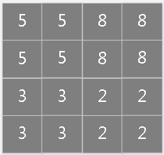
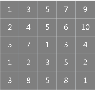
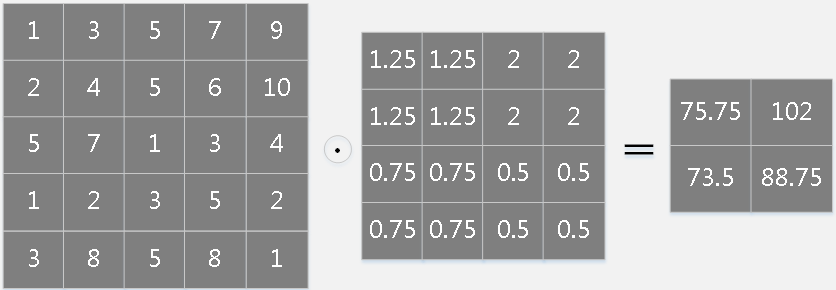
2、当前层为卷积层,与其相连的上一层相关核权重及偏置计算如下:
假设通过\((p,q)\)来标识卷积层任意位置,则:
\[ \begin{array}{l} \frac{\partial E}{\partial k_{ij}^n} =\sum_{p,q}(\delta_j^{n})_{pq}(X_{i}^{n-1})_{pq}\\ \frac{\partial E}{\partial b_j}=\sum_{p,q}(\delta_j^{n})_{pq} \end{array} \] 假设第\(n-1\)层输入矩阵大小为5×5:
![]()
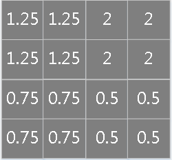
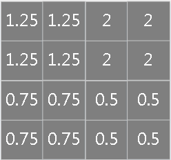
第\(n\)层误差敏感项矩阵大小为4×4:
![]()
则核\(k_{ij}^n\)的偏导为:
![]()
\[ \begin{aligned} 75.75=&1*1.25+3*1.25+5*2+7*2+\\ &2*1.25+4*1.25+5*2+6*2+\\ &5*0.75+7*0.75+1*0.5+3*0.5+\\ &1*0.75+2*0.75+3*0.5+5*0.5 \end{aligned} \]
偏置\(b_j\)的偏导为误差敏感项矩阵元素之和: \[ \begin{aligned} 18=1.25*4+0.75*4+2*4+0.5*4 \end{aligned} \]
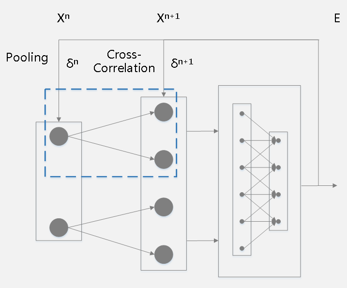
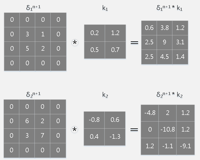
3、当前层为下采样(pooling)层且下一层为卷积层时反向传播的原理如下: \[ \begin{array}{l} \delta^n_j=F'(Y_j^n)\sum_{p,q}(\delta_j^{n+1})_{pq}*(k_{j}^{n+1})_{pq}\\ \end{array} \]
其中运算符号\(*\)为卷积操作。一个简单的例子如下:
![]()
假设下采样(pooling)层处于第\(n\)层且feature map大小为3×3,其下一层为卷积层处于第\(n+1\)层且通过两个2×2卷积核得到了两个feature map(蓝色虚框框住的网络结构)。
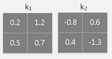
2个卷积核为:
![]()
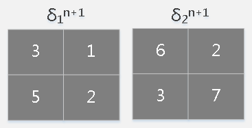
假设第\(n+1\)层对两个卷积核的误差敏感项已经计算好:
![]()
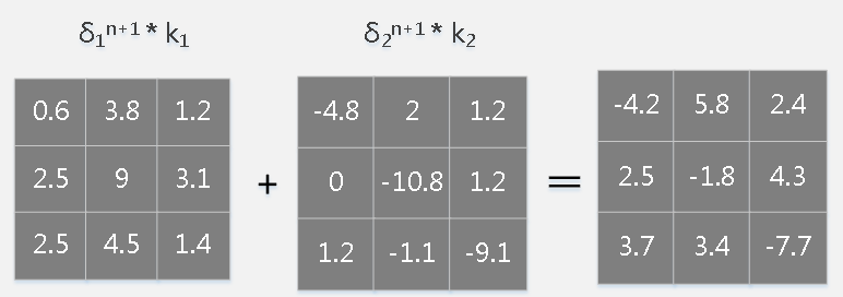
则对第\(n+1\)层的误差敏感项做zero-padding并利用卷积操作(注意:会对卷积核做180度旋转)可以得到第\(n\)层的误差敏感项,过程如下:
![]()
假设\(F'(Y_j^n)=1\),则第\(n\)层的误差敏感项为:
![]()
5.3.8 CNN在NLP领域应用实例
在NLP领域,文本分类是一类常用应用,传统方法是人工提取类似n-gram的各种特征以及各种交叉组合。文本类似图像天然有一种局部相关性,想到利用CNN做一种End to End的分类器,把提特征的工作交给模型。
对于一个句子,它是一维的,无法像图像一样直接处理,因此需要通过distributed representation learning得到词向量,或者在模型第一层增加一个embedding层起到类似作用,这样一个句子就变成二维的了:
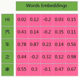
我们用Tensorflow为后端的Keras搭建这个模型:
前面说到可以使用两种方法得到词向量:
1、预先训练好的结果,例如使用已经训练好的word2vec模型,相关资料:Using pre-trained word embeddings in a Keras model;
2、模型第一层增加embedding层,我们使用这种方式。
网络结构如下:
1 | def build_embedding_cnn(max_caption_len, vocab_size): |
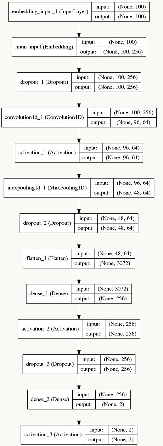
详细代码可以参见GitHub:Cnn-tc-Keras。
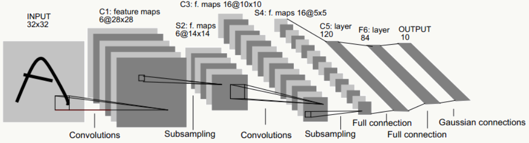
5.4 LeNet-5
最初的网络结构来源于论文:《Gradient-based learning applied to document recognition》(论文里使用原始未做规范化的数据时,INPUT是32×32的),我用以下结构做说明: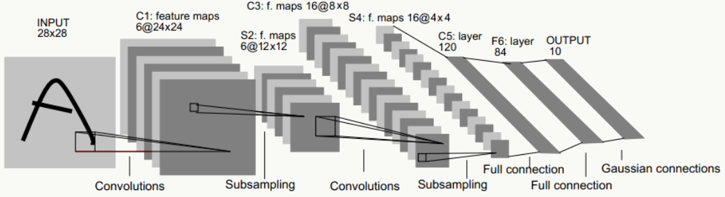
LeNet-5一共有8层:1个输入层+3个卷积层(C1、C3、C5)+2个下采样层(S2、S4)+1个全连接层(F6)+1个输出层,每层有多个feature map(自动提取的多组特征)。
5.4.1 输入层
采用keras自带的MNIST数据集,输入像素矩阵为28×28的单通道图像数据。
5.4.2 C1卷积层
由6个feature map组成,每个feature map由5×5卷积核生成(feature map中每个神经元与输入层的5×5区域像素相连),考虑每个卷积核的bias,该层需要学习的参数个数为:(5×5+1)×6=156个,神经元连接数为:156×24×24=89856个。
5.4.3 S2下采样层
该层每个feature map一一对应上一层的feature map,由于每个单元的2×2感受野采用不重叠方式移动,所以会产生6个大小为12×12的下采样feature map,如果采用Max Pooling/Mean Pooling,则该层需要学习的参数个数为0个(如果采用非等权下采样——即采样核有权重,则该层需要学习的参数个数为:(2×2+1)×6=30个),神经元连接数为:30×12×12=4320个。
5.4.4 C3卷积层
这层略微复杂,S2神经元与C3是多对多的关系,比如最简单方式:用S2的所有feature map与C3的所有feature map做全连接(也可以对S2抽样几个feature map出来与C3某个feature map连接),这种全连接方式下:6个S2的feature map使用6个独立的5×5卷积核得到C3中1个feature map(生成每个feature map时对应一个bias),C3中共有16个feature map,所以该层需要学习的参数个数为:(5×5×6+1)×16=2416个,神经元连接数为:2416×8×8=154624个。
5.4.5 S4下采样层
同S2,如果采用Max Pooling/Mean Pooling,则该层需要学习的参数个数为0个,神经元连接数为:(2×2+1)×16×4×4=1280个。
5.4.6 C5卷积层
类似C3,用S4的所有feature map与C5的所有feature map做全连接,这种全连接方式下:16个S4的feature map使用16个独立的1×1卷积核得到C5中1个feature map(生成每个feature map时对应一个bias),C5中共有120个feature map,所以该层需要学习的参数个数为:(1×1×16+1)×120=2040个,神经元连接数为:2040个。
5.4.7 F6全连接层
将C5层展开得到4×4×120=1920个节点,并接一个全连接层,考虑bias,该层需要学习的参数和连接个数为:(1920+1)*84=161364个。
5.4.8 输出层
该问题是个10分类问题,所以有10个输出单元,通过softmax做概率归一化,每个分类的输出单元对应84个输入。
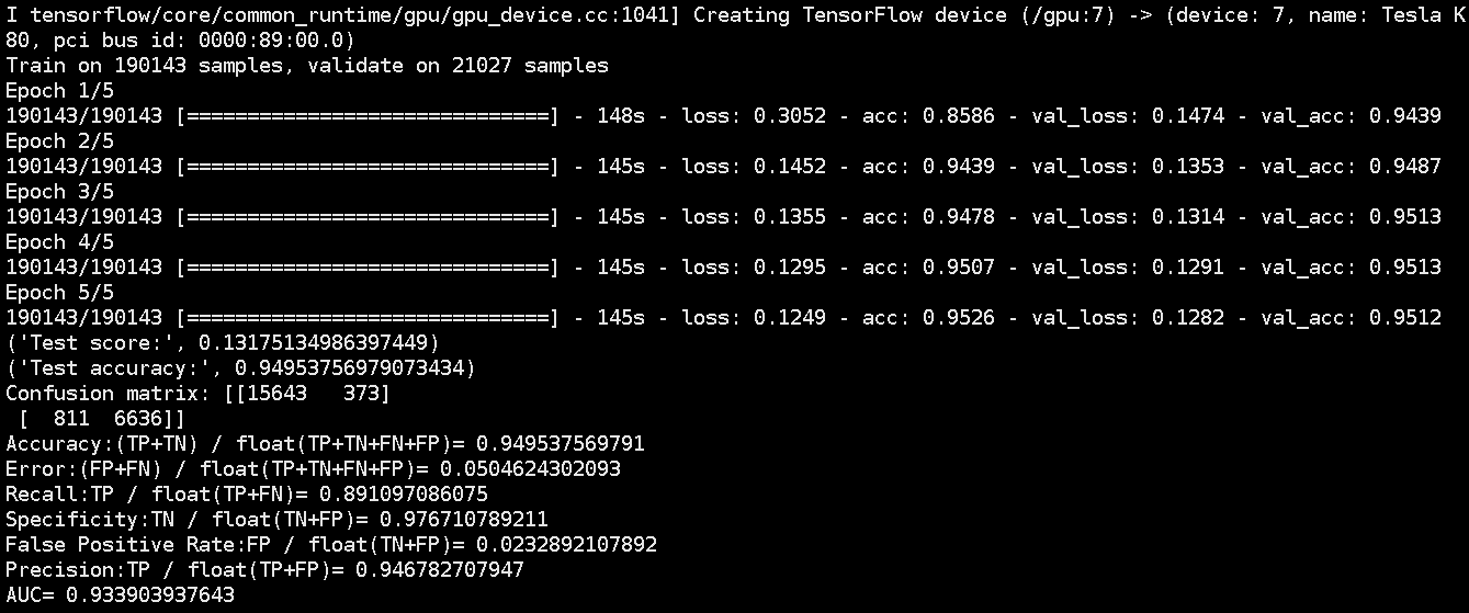
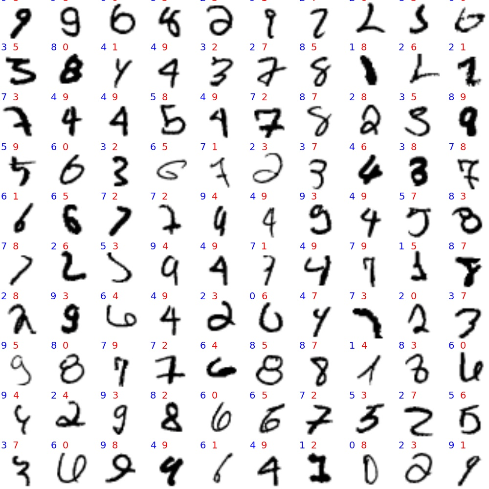
Minist(Modified NIST)数据集下使用LeNet-5的训练可视化: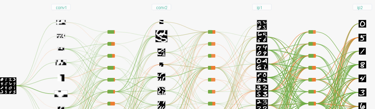
可以看到其实全连接层之前的各层做的就是特征提取的事儿,且比较通用,对于标准化实物(人、车、花等等)可以复用,后面会单独介绍模型的fine-tuning。
5.4.9 LeNet-5代码实践
1 | import copy |
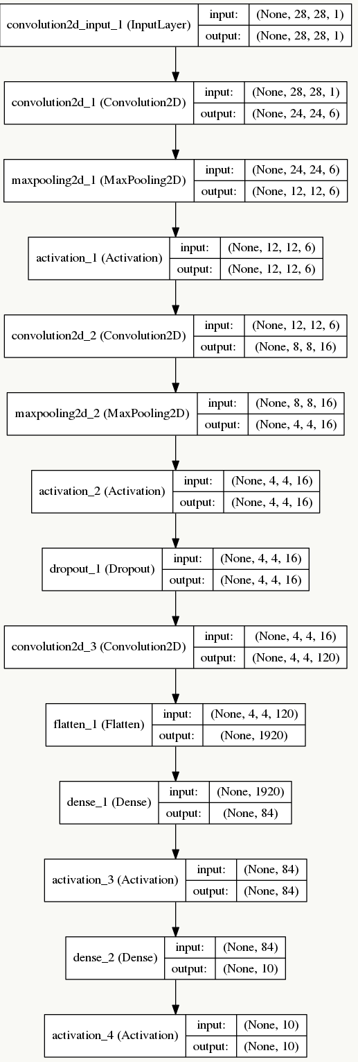
- 网络结构
![]()
- 错误分类可视化
![]()
5.5 AlexNet
AlexNet在ILSVRC-2012的比赛中获得top5错误率15.3%的突破(第二名为26.2%),其原理来源于2012年Alex的论文《ImageNet Classification with Deep Convolutional Neural Networks》,这篇论文是深度学习火爆发展的一个里程碑和分水岭,加上硬件技术的发展,深度学习还会继续火下去。
5.5.1 网络结构分析
由于受限于当时的硬件设备,AlexNet在GPU粒度都做了设计,当时的GTX 580只有3G显存,为了能让模型在大量数据上跑起来,作者使用了两个GPU并行,并对网络结构做了切分,如下: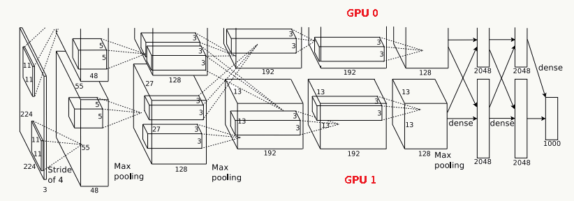
上下两层分别并行的跑在两个GPU上,虚线代表依赖,交叉的虚线代表两个GPU之间需要通信后交换数据。
输入层
输入为224×224×3的三通道RGB图像,为方便后续计算,实际操作中通过padding做预处理,把图像变成227×227×3。
C1卷积层
该层由:卷积操作 + Max Pooling + LRN(后面详细介绍它)组成。
(1)、卷积层:由96个feature map组成,每个feature map由11×11卷积核在stride=4下生成,输出feature map为55×55×48×2,其中55=(227-11)/4+1,48为分在每 个GPU上的feature map数,2为GPU个数;
(2)、激活函数:采用ReLU;
(3)、Max Pooling:采用stride=2且核大小为3×3(文中实验表明采用2×2的非重叠模式的Max Pooling相对更容易过拟合,在top 1和top 5下的错误率分别高0.4%和0.3%),输出feature map为27×27×48×2,其中27=(55-3)/2+1,48为分在每个GPU上的feature map数,2为GPU个数;
(4)、LRN:邻居数设置为5做归一化。 最终输出数据为归一化后的:27×27×48×2。
C2卷积层
该层由:卷积操作 + Max Pooling + LRN组成
(1)、卷积层:由256个feature map组成,每个feature map由5×5卷积核在stride=1下生成,为使输入和卷积输出大小一致,需要做参数为2的padding,输出feature map为27×27×128×2,其中27=(27-5+2×2)/1+1,128为分在每个GPU上的feature map数,2为GPU个数;
(2)、激活函数:采用ReLU;
(3)、Max Pooling:采用stride=2且核大小为3×3,输出feature map为13×13×128×2,其中13=(27-3)/2+1,128为分在每个GPU上的feature map数,2为GPU个数;
(4)、LRN:邻居数设置为5做归一化。
最终输出数据为归一化后的:13×13×128×2。
C3卷积层 该层由:卷积操作 + LRN组成(注意,没有Pooling层)
(0)、输入为13×13×256,因为这一层两个GPU会做通信(途中虚线交叉部分)
(1)、卷积层:之后由384个feature map组成,每个feature map由3×3卷积核在stride=1下生成,为使输入和卷积输出大小一致,需要做参数为1的padding,输出feature map为13×13×192×2,其中13=(13-3+2×1)/1+1,192为分在每个GPU上的feature map数,2为GPU个数;
(2)、激活函数:采用ReLU;
最终输出数据为归一化后的:13×13×192×2。
C4卷积层 该层由:卷积操作 + LRN组成(注意,没有Pooling层)
(1)、卷积层:由384个feature map组成,每个feature map由3×3卷积核在stride=1下生成,为使输入和卷积输出大小一致,需要做参数为1的padding,输出feature map为13×13×192×2,其中13=(13-3+2×1)/1+1,192为分在每个GPU上的feature map数,2为GPU个数;
(2)、激活函数:采用ReLU; 最终输出数据为归一化后的:13×13×192×2。
C5卷积层 该层由:卷积操作 + Max Pooling组成
(1)、卷积层:由256个feature map组成,每个feature map由3×3卷积核在stride=1下生成,为使输入和卷积输出大小一致,需要做参数为1的padding,输出feature map为13×13×128×2,其中13=(13-3+2×1)/1+1,128为分在每个GPU上的feature map数,2为GPU个数;
(2)、激活函数:采用ReLU;
(3)、Max Pooling:采用stride=2且核大小为3×3,输出feature map为6×6×128×2,其中6=(13-3)/2+1,128为分在每个GPU上的feature map数,2为GPU个数. 最终输出数据为归一化后的:6×6×128×2。
F6全连接层 该层为全连接层 + Dropout
(1)、使用4096个节点;
(2)、激活函数:采用ReLU;
(3)、采用参数为0.5的Dropout操作
最终输出数据为4096个神经元节点。
F7全连接层 该层为全连接层 + Dropout
(1)、使用4096个节点;
(2)、激活函数:采用ReLU;
(3)、采用参数为0.5的Dropout操作
最终输出为4096个神经元节点。
F8输出层 该层为全连接层 + Softmax
(1)、使用1000个输出的Softmax
最终输出为1000个分类。
AlexNet的亮点如下:
5.5.2 ReLu激活函数
AlexNet引入了ReLU激活函数,这个函数是神经科学家Dayan、Abott在《Theoretical Neuroscience》一书中提出的更精确的激活模型: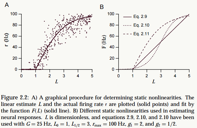
其中: \[ \begin{array}{l} \text{Eq.2.9: }F(L)=G[L-L_0]_+\\ \text{Eq.2.10: }F(L)=\frac{r_{max}}{1+exp(g_1(L_{1/2}-L))}\\ \text{Eq.2.11: }F(L)=r_{max}[tanh (g_2(L-L_0))]_+ \end{array} \]
详情请阅读书中2.2 Estimating Firing Rates这一节。新激活模型的特点是:
激活稀疏性(\(L\)小于1时\(r\)为0)
单边抑制(不像Sigmoid是双边的)
宽兴奋边界,非饱和性(ReLU导数始终为1),很大程度缓解了梯度消失问题
1、 原始ReLu
在这些前人研究的基础上(可参见 Hinton论文:《Rectified Linear Units Improve Restricted Boltzmann Machines》),类似Eq.2.9的新激活函数被引入: \[f(x)=max(0,x)\] 这个激活函数把负激活全部清零(模拟上面提到的稀疏性),这种做法在实践中即保留了神经网络的非线性能力,又加快了训练速度。 但是这个函数也有缺点:
在原点不可微
反向传播的梯度计算中会带来麻烦,所以Charles Dugas等人又提出Softplus来模拟上述ReLu函数(可视作其平滑版): \[f(x)=log(1+e^x)\]
实际上它的导数就是一个logistic-sigmoid函数: \[f’(x)=\frac{1}{1+e^{-x}}\]
过稀疏性 当学习率设置不合理时,即使是一个很大的梯度,在经过ReLu单元并更新参数后该神经元可能永不被激活。
2、 Leaky ReLu
为了解决上述过稀疏性导致的大量神经元不被激活的问题,Leaky ReLu被提了出来: \[ f(x)=\left\{ \begin{aligned} \alpha x &(x<0) \\ x &(x>=0) \end{aligned} \right. \] 其中\(\alpha\)是人工指定的较小值(如:0.1),它一定程度保留了负激活信息。
3、Parametric ReLu 上述\(\alpha\)值是可以不通过人为指定而学习出的,于是Parametric ReLu被提了出来: 利用误差反向传播原理: \[ \begin{array}{l} \frac{\partial{E}}{\partial{\alpha}}=\sum\frac{\partial{E}}{\partial{f(x)}}\frac{\partial{f(x)}}{\partial{\alpha}} \end{array} \] \[ \frac{\partial{f(x)}}{\partial{\alpha}}=\left\{ \begin{aligned} x &(x<0) \\ 0 &(x>=0) \end{aligned} \right. \] 当采用动量法更新\(\alpha\)权重: \[ \Delta\alpha=\mu\Delta\alpha+\epsilon\frac{\partial{E}}{\partial{\alpha}} \] 详情请阅读Kaiming He等人的《Delving Deep into Rectifiers: Surpassing Human-Level Performance on ImageNet Classification》论文。
4、Randomized ReLu Randomized ReLu 可以看做是leaky ReLu的随机版本,原理是:假设\[\alpha\text{~}Normal(\mu,\delta)\]然后再做权重调整。 \[ f(x)=\left\{ \begin{aligned} \alpha x &(x<0) \\ x &(x>=0) \end{aligned} \right. \] 其中:\[ \alpha\text{~}Normal(\mu,\delta)\text{ and }\mu<\delta\text{ and }\mu,\delta\in[0,1)\]
5.5.3 Local Response Normalization
LRN利用相邻feature map做特征显著化,文中实验表明可以降低错误率,公式如下: \[ \begin{array}{l} b_{x,y}^i=a_{x,y}^i/(k+\alpha \sum_{j=max(0,i-n/2)}^{min(N-1,i+n/2)}(a^i_{x,y})^2)^\beta \end{array} \]
公式的直观解释如下: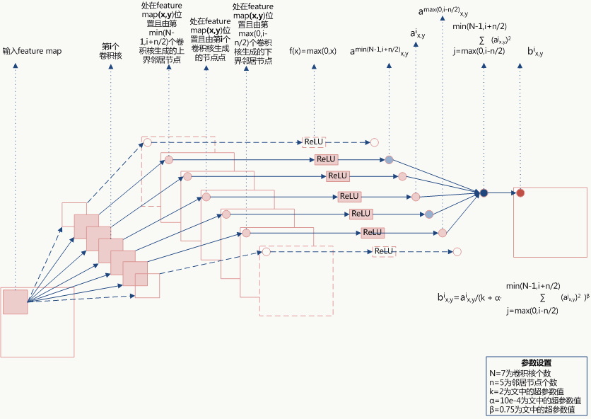
当\(\sum x^2\)值较小时,即当前节点和其邻居节点输出值差距不明显且大家的输出值都不太大,可以认为此时特征间竞争激烈,该函数可以使原本差距不大的输出产生显著性差异且此时函数输出不饱和;当\(\sum x^2\)值较大时,说明特征本身有显著性差别但输出值太大容易过拟合,该函数可以令最终输出接近0从而缓解过拟合提高了模型泛化性。
5.5.4 Overlapping Pooling
如其名,实验表明有重叠的抽样可以提高泛化性。
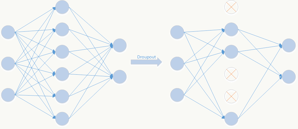
5.5.5 Dropout
Dropout是文章亮点之一,属于提高模型泛化性的方法,操作比较简单,以一定概率随机让某些神经元输出设置为0,既不参与前向传播也不参与反向传播,也可以从正则化角度去看待它。
- 从模型集成的角度看
![]()
无Dropout网络: \[ \begin{array}{l} Y^n=W^nX^{n-1}\\ X^n=F(Y^n)\\ \end{array} \]
有Dropout网络: \[ \begin{array}{l} Y^n=W^nX^{n-1}\\ d^{n-1}\sim Bernoulli (p)\\ X^n=d^{n-1} \odot F(Y^n) \end{array} \] 其中\(p\)为Dropout的概率,\(n\)为所在层。
它是极端情况下的Bagging,由于在每步训练中,神经元会以某种概率随机被置为无效,相当于是参数共享的新网络结构,每个模型为了使损失降低会尽可能学最“本质”的特征,“本质”可以理解为由更加独立的、和其他神经元相关性弱的、泛化能力强的神经元提取出来的特征;而如果采用类似SGD的方式训练,每步迭代都会选取不同的数据集,这样整个网络相当于是用不同数据集学习的多个模型的集成组合。
从数据扩充(Data Augmentation)的角度看:
机器学习学的就是原始数据的数据分布,而泛化能力强的模型自然不能只针对训练集上的数据正确映射输出,但要想学到好的映射又需要数据越多越好,很多论文已经证明,带领域知识的数据扩充能够提高训练数据对原始真实分布的覆盖度,从而能够提高模型泛化效果。 《Dropout as Data Augmentation》将Dropout看做数据扩充的方法,文中证明了:总能找到一个样本,使得原始神经网络的输出与Dropout神经网络的输出一致(projecting noise back into the input space)。 用论文中符号说明如下: \[ \begin{array}{l} h(x)=xW+b\\ a(h)=rect(h)\\ \widetilde{a}(h)=M \odot rect(h) \end{array} \] 其中:\(x\)为\(d_i\)维空间的输入,\(h(x)\)为从\(d_i\)维空间到\(d_h\)维空间的仿射映射,\(a(h)\)为激活函数,\(\widetilde{a}(h)\)为Dropout版激活函数,\(M\sim Bernoulli(p_h)\),\(rect(h)\)为rectifier函数(比如:ReLU): 对任何一个隐层,假设都存在一个输入\(x^*\),满足: \[ (a\circ h)(x^*)=rect(h(x^*))\approx \vec{m}\odot rect(h(x))=(\widetilde{a} \circ h)(x) \] 注:式子左边为原始神经网络某层,右边为Dropout神经网络某层。 采用SGD优化下面目标函数,总能找到一个输入\(x^*\): \[min~L(x,x^*)=min~|(a\circ h)(x^*)-(\widetilde{a} \circ h)(x)|^2\]
对于一个\(n\)层的神经网络: 原始神经网络表示为: \[ {f}^{(i)}(x^*)=({a}^{(i)}\circ h^{(i)}\circ ...\circ{a}^{(1)}\circ h^{(1)})(x^*) \]
Dropout神经网络表示为: \[ \widetilde{f}^{(i)}(x)=(\widetilde{a}^{(i)}\circ h^{(i)}\circ ...\circ\widetilde{a}^{(1)}\circ h^{(1)})(x) \]
采用SGD优化下面目标函数,总能找到一系列输入\((x^{(1)*},...,x^{(n)*})\): \[ min~L(x,x^{(1)*},...,x^{(n)*})=min~\sum_{i=1}^{n}\lambda_i|{f}^{(i)}(x^{(i)*})-\widetilde{f}^{(i)}(x)|^2 \]
文中附录部分证明不可能找到唯一序列使得:\(x^*=x^{(1)*}=...=x^{(n)*}\)
所以每次Dropout都是在生成新的样本。
5.5.6 数据扩充
基本方法 正如前面所说,数据扩充本质是减少过拟合的方法,AlexNet使用的方法计算量较小,所以也不用存储在磁盘,代码实现时,当GPU在训练前一轮图像时,后一轮的图像扩充在CPU上完成,扩充使用了两种方法:
1、图像平移和图像反射(关于某坐标轴对称);
2、通过ImageNet训练集做PCA,用PCA产生的特征值和特征向量及期望为0标准差为0.1的高斯分布改变原图RGB三个通道的强度,该方法使得top-1错误率降低1%。
5.5.7 多GPU训练
作者使用GTX 580来加速训练,但受限于当时硬件设备的发展,作者需要对网络结构做精细化设计,甚至需要考虑两块GPU之间如何及何时通信,现在的我们比较幸福,基本不用考虑这些。
5.5.8 AlexNet代码实践
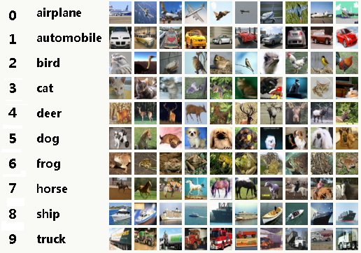
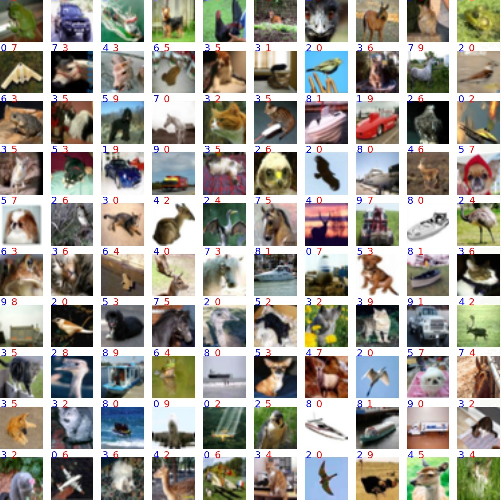
使用CIFAR-10标准数据集,由6w张32×32像素图片组成,一共10个分类。像这样:
代码实现:
1 | # -*- coding: utf-8 -*- |
- 训练数据可视化
- 网络结构
![]()
可以看到实践中,AlexNet的参数规模巨大(将近2亿个参数),所以即使在GPU上训练也很慢。
错误分类可视化
蓝色为实际分类,红色为预测分类。
5.6 VGG
在论文《Very Deep Convolutional Networks for Large-Scale Image Recognition》中提出,通过缩小卷积核大小来构建更深的网络。
5.6.1 网络结构
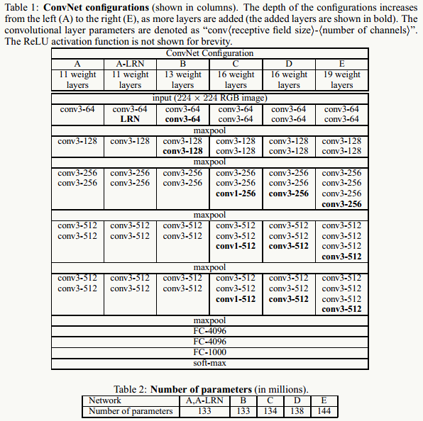
图中D和E分别为VGG-16和VGG-19,是文中两个效果最好的网络结构,VGG网络结构可以看做是AlexNet的加深版,VGG在图像检测中效果很好(如:Faster-RCNN),这种传统结构相对较好的保存了图片的局部位置信息(不像GoogLeNet中引入Inception可能导致位置信息的错乱)。 与AlexNet相比:
相同点
整体结构分五层;
除softmax层外,最后几层为全连接层;
五层之间通过max pooling连接。
不同点
使用3×3的小卷积核代替7×7大卷积核,网络构建的比较深;
由于LRN太耗费计算资源,性价比不高,所以被去掉;
采用了更多的feature map,能够提取更多的特征,从而能够做更多特征的组合。
5.6.2 VGG代码实践
VGG-16/VGG-19
使用CIFAR-100数据集,ps复杂网络在这种数据集上表现不好。
1 | # -*- coding: utf-8 -*- |
5.7 MSRANet
该网络的亮点有两个:提出PReLU和一种鲁棒性强的参数初始化方法
5.7.1 PReLU
前面已经介绍过传统ReLU的一些缺点,PReLU是其中一种解决方案: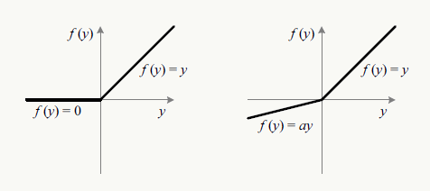
如何合理保留负向信息,一种方式是上图中\(\alpha\)值是可以不通过人为指定而自动学出来:
定义Parametric Rectifiers如下: \[ f(y_i)=\left\{ \begin{aligned} y_i, & \text{if } y_i>0 \\ \alpha_i y_i, & else. \end{aligned} \right. \] 利用误差反向传播原理: \[ \begin{array}{l} \frac{\partial{E}}{\partial{\alpha_i}}=\sum_{y_i}\frac{\partial{E}}{\partial{f(y_i)}}\frac{\partial{f(y_i)}}{\partial{\alpha_i}} \end{array} \] \[ \frac{\partial{f(y_i)}}{\partial{\alpha_i}}=\left\{ \begin{aligned} y_i, &(y_i\leq 0) \\ 0, &(y_i>0) \end{aligned} \right. \] 当采用动量法更新\(\alpha\)权重: \[ \Delta\alpha_i=\mu\Delta\alpha_i+\epsilon\frac{\partial{E}}{\partial{\alpha_i}} \] 详情请阅读Kaiming He等人的《Delving Deep into Rectifiers: Surpassing Human-Level Performance on ImageNet Classification》论文。
5.8 Highway Networks
Highway Networks在我看来是一种承上启下的结构,来源于论文《Highway Networks》借鉴了类似LSTM(后面会介绍)中门(gate)的思想,结构很通用(太通用的结构不一定是件好事儿),给出了一种建立更深网络的思路: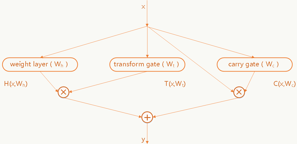
\[ \begin{array}{l} y=H(x,W_h)\cdot T(x,W_t)+x \cdot C(x,W_c) \end{array} \] 任何一层或几层都可以通过上述方式构建Block,公式中\(T\)叫做transform gate,\(C\)叫做carry gate,一般简单起见可以让\(C=1-T\),显然公式中\(x\),\(y\),\(H(x,W_h)\),\(T(x,W_t)\)需要有相同的维度(比如,可以通过zero-padding或者做映射),通过这种结构可以把网络做到很深(比如100层以上),并且优化没有那么困难,看着似乎提供了解决“深”网络学习问题的方案(下一节会解释“似乎”这个词)。
5.9 Residual Networks
残差网络在《Deep Residual Learning for Image Recognition》中被第一次提出,作者利用它在ILSVRC 2015的ImageNet 分类、检测、定位任务以及COCO 2015的检测、图像分割任务上均拿到第一名,也证明ResNet是比较通用的框架。
5.9.1 ResNet产生的动机
我一直说深度学习的研究很大程度是实验科学,ResNet的研究上也比较能体现这点。一个问题:是否能够通过简单的增加网络层数就能学到更好的模型呢?通过实验发现答案是否定的,并且随着层数的增加预测精度会趋于饱和,然后迅速下降,这个现象叫degradation。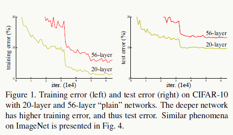
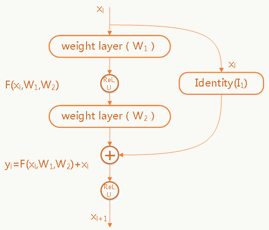
\[ \begin{array}{l} y_l=h(x_l)+F(x_l,\{W_l\})\\ x_{l+1}=f(y_l) \end{array} \] 其中\(h(x_l)=x_l\)为恒等映射,\(f\)为\(ReLU\)激活函数,输入和输出的维度是一样的(即使不一样也可以通过zero-padding或再做一次映射变成一样),图中恒等映射是在两层神经网络后,也可以在任意层后。 这个框架的假设是:多层非线性激活的神经网络学习恒等映射的能力比较弱,直接将恒等映射加入可以跳过这个问题。 与Highway Networks相比: - HN的transform gate和carry
5.9.2 恒等映射
恒等映射在深度残差网络中究竟扮演什么角色呢?在《Identity Mappings in Deep Residual Networks》中作者做了分析,并提出新的残差block结构,将\(h(x_l)=x_l\)和\(f(y_l)=y_l\)都改为恒等映射,通过这个变化使得信号在前向和反向传播中都有“干净”的路径(图中灰色部分),a为原始block结构,b为新的结构。。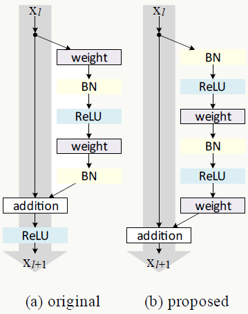
原始结构: \[ \begin{array}{l} x_{l+1}=relu(B(W_{i2}^T\cdot relu (B(W_{i1}^T\cdot x_l)))+x_l) \end{array} \]
新结构: \[ \begin{array}{l} x_{l+1}=W_{i2}^T\cdot relu(B(W_{i1}^T\cdot relu(B(x_l))))+x_l \end{array} \]
其中\(B\)为Batch Normalization。
在CIFAR-10上用1001层残差网络做测试,效果如下: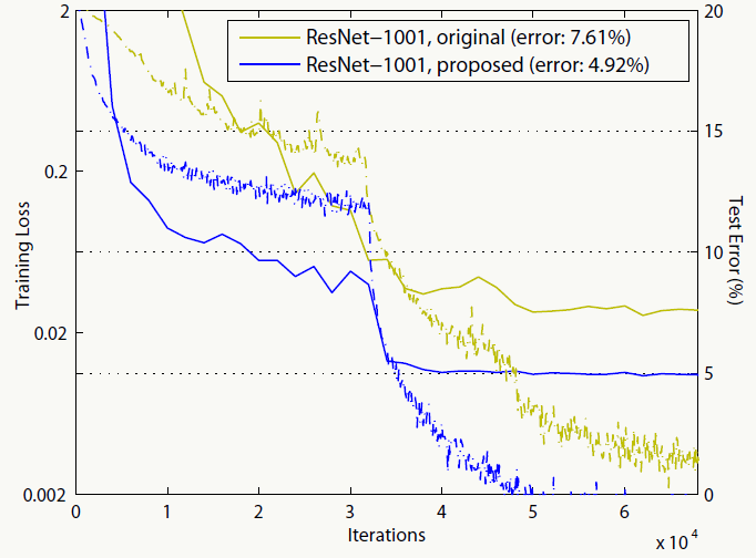
新的proposed结构比原始结构效果明显: 双恒等映射下,任何一个残差block如下: \[ \begin{array}{l} x_{l+1}=x_l+F(x_l,\{W_l\}) \end{array} \] 对上述结构做递归展开,任何一个深层block和其所有浅层block的关系为: \[ \begin{array}{l} x_L=x_l+\sum_{i=l}^{L-1}F(x_i,\{W_i\})\\ x_L=x_0+\sum_{i=0}^{L-1}F(x_i,\{W_i\}) \end{array} \] 这个形式会有很好的计算性质,回想GBDT,是否觉得有点像?在反向传播时同样也有良好的性质: \[ \begin{array}{l} \frac{\partial E}{\partial x_l}=\frac{\partial E}{\partial x_L}\frac{\partial x_L}{\partial x_l}=\frac{\partial E}{\partial x_L}(1+\frac{\partial}{\partial x_l}\sum_{i=l}^{L-1}F(x_i,\{W_i\})) \end{array} \] 前半部分\(\frac{\partial E}{\partial x_L}\)传播时完全不用考虑权重层,可以很直接的把误差的梯度信息反向传播给任何一个浅层block,而\(\frac{\partial}{\partial x_l}\sum_{i=l}^{L-1}F(x_i,\{W_i\})\)在mini-batch时又不太可能总为-1,所以即使权重很小也很难出现梯度消失的问题。假如不采用恒等映射,例如:\(h(x_l)=\lambda_lx_l\),则: \[ \begin{array}{l} x_{l+1}=\lambda_lx_l+F(x_l,\{W_l\})\\ x_L=(\prod_{i=1}^{L-1}\lambda_i)x_l+\sum_{i=l}^{L-1}(\prod_{j=i+1}^{L-1}\lambda_j)F(x_i,\{W_i\})\\ \frac{\partial E}{\partial x_l}=\frac{\partial E}{\partial x_L}(\prod_{i=1}^{L-1}\lambda_i+\frac{\partial}{\partial x_l}\sum_{i=l}^{L-1}(\prod_{j=i+1}^{L-1}\lambda_j)F(x_i,\{W_i\})) \end{array} \] 如果网络比较深,对于参数\(\prod_{i=1}^{L-1}\lambda_i\),当\(\lambda_i>1\)时它会很大;当\(\lambda_i<1\)时,它会很小甚至消失,此时反向信号会被强制流到block的各个权重层,显然恒等映射的优点完全没有了。
5.9.3 模型集成角度看残差网络
《Residual Networks Behave Like Ensembles of Relatively Shallow Networks》中把残差网络做展开,其实会发现以下关系: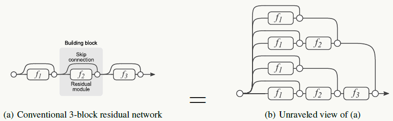
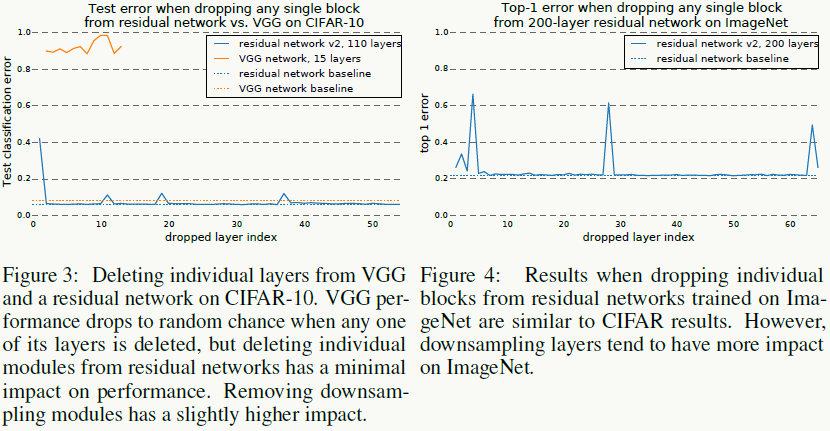
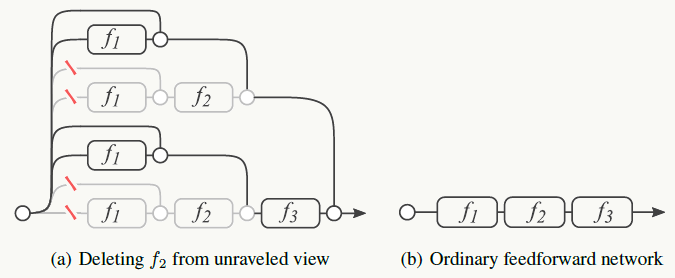
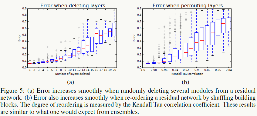
模型在运行时的效果与有效路径的个数成正比且关系平滑,左图说明残差网络的效果类似集成模型,右图说明实践中残差网络可以在运行时做网络结构修改。
5.9.4 残差网络中的短路径
通过残差block的结构可知展开后的\(n\)个路径的长度服从二项分布\(X\sim B(n,1/2)\),(每次选择是否跳过权重层的概率是0.5),所以其期望为:\(n/2\),下面三幅图是在有54个残差block下的实验,第一幅图为路径分布图,可以看到95%的路径长度都在19~35之间: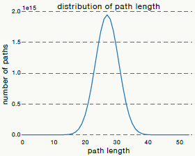
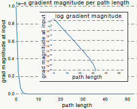
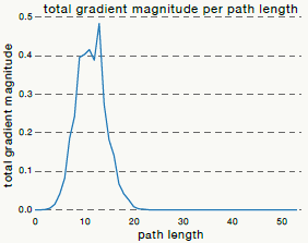
虽然残差网络没有解决梯度消失问题,只是把它给绕过了,并没有解决深层神经网络的本质问题,但我们应用时更多的看实践效果。
5.9.5 代码实践
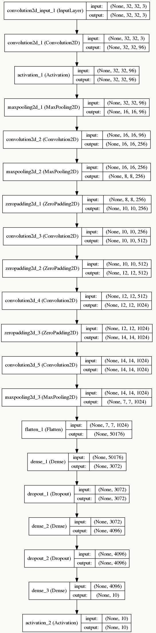
下面我们实现在《Deep Residual Learning for Image Recognition》中提到的ResNet-34,并演示在CIFAR-10下的训练效果。
resnet.py
1
2
3
4
5
6
7
8
9
10
11
12
13
14
15
16
17
18
19
20
21
22
23
24
25
26
27
28
29
30
31
32
33
34
35
36
37
38
39
40
41
42
43
44
45
46
47
48
49
50
51
52
53
54
55
56
57
58
59
60
61
62
63
64
65
66
67
68
69
70
71
72
73
74
75
76
77
78
79
80
81
82
83
84
85
86
87
88
89
90
91
92
93
94
95
96
97
98
99
100
101
102
103
104
105
106
107
108
109
110
111
112
113
114
115
116
117
118
119
120
121
122
123
124
125
126
127
128
129
130
131
132
133
134
135
136
137
138
139
140
141
142
143
144
145
146
147
148
149
150
151
152
153# -*- coding: utf-8 -*-
from keras import backend as K
from keras.layers.merge import add
from keras.layers import Input, Activation, Dense, Flatten
from keras.layers.convolutional import Conv2D, MaxPooling2D, AveragePooling2D
from keras.layers.normalization import BatchNormalization
from keras.regularizers import l1_l2
from keras.models import Model
class ResNet(object):
'''残差网络基本模块定义'''
name = 'resnet'
def __init__(self, n):
self.name = n
def bn_relu(self, input):
'''构建propoesd残差block中BN与ReLU子结构,针对tensorflow'''
normalize = BatchNormalization(axis=3)(input)
return Activation("relu")(normalize)
def bn_relu_weight(self, filters, kernel_size, strides):
'''构建propoesd残差block中BN->ReLu->Weight的子结构'''
def inner_func(input):
act = self.bn_relu(input)
conv = Conv2D(filters=filters,
kernel_size=kernel_size,
strides=strides,
padding='same',
kernel_initializer='he_normal',
kernel_regularizer=l1_l2(0.0001))(act)
return conv
return inner_func
def weight_bn_relu(self, filters, kernel_size, strides):
'''构建propoesd残差block中BN->ReLu->Weight的子结构'''
def inner_func(input):
return self.bn_relu(Conv2D(filters=filters,
kernel_size=kernel_size,
strides=strides,
padding='same',
kernel_initializer='he_normal',
kernel_regularizer=l1_l2(0.0001))(input))
return inner_func
def shortcut(self, left, right):
'''构建propoesd残差block中恒等映射的子结构,分两种情况,输入、输出维度一致&维度不一致'''
left_shape = K.int_shape(left)
right_shape = K.int_shape(right)
stride_width = int(round(left_shape[1] / right_shape[1]))
stride_height = int(round(left_shape[2] / right_shape[2]))
equal_channels = left_shape[3] == right_shape[3]
x_l = left
# 如果输入输出维度不一致需要通过映射变一致,否则一致则返回单位矩阵,这个映射发生在两个不同维度block之间(论文中虚线部分)
if left_shape != right_shape:
x_l = Conv2D(filters=right_shape[3],
kernel_size=(1, 1),
strides=(int(round(left_shape[1] / right_shape[1])),
int(round(left_shape[2] / right_shape[2]))),
padding="valid",
kernel_initializer="he_normal",
kernel_regularizer=l1_l2(0.01, 0.0001))(left)
x_l_1 = add([x_l, right])
return x_l_1
def basic_block(self, filters, strides=(1, 1), is_first_block=False):
"""34层以内的残差网络使用的block,2层一跨"""
def inner_func(input):
# 恒等映射
if not is_first_block:
conv1 = self.bn_relu_weight(filters=filters,
kernel_size=(3, 3),
strides=strides)(input)
else:
conv1 = Conv2D(filters=filters, kernel_size=(3, 3),
strides=strides,
padding="same",
kernel_initializer="he_normal",
kernel_regularizer=l1_l2(0.01, 0.0001))(input)
# 残差网络
residual = self.bn_relu_weight(filters=filters,
kernel_size=(3, 3), strides=(1, 1))(conv1)
# 构建一个两层的残差block
return self.shortcut(input, residual)
return inner_func
def residual_block(self, block_func, filters, repeat_times, is_first_block):
'''构建多层残差block'''
def inner_func(input):
for i in range(repeat_times):
# 第一个block的第一层,其输入为pooling层
if is_first_block:
strides = (1, 1)
else:
if i == 0: # 每个残差block的第一层
strides = (2, 2)
else: # 每个残差block的非第一层
strides = (1, 1)
flag = i == 0 and is_first_block
input = block_func(filters=filters,
strides=strides,
is_first_block=flag)(input)
return input
return inner_func
def residual_builder(self, input_shape, softmax_num, func_type, repeat_times):
'''指定输入、输出、残差block的类型、网络深度并构建残差网络'''
input = Input(shape=input_shape)
# 第一层为卷积层
conv1 = self.weight_bn_relu(filters=64, kernel_size=(7, 7), strides=(2, 2))(input)
# 第二层为max pooling层
pool1 = MaxPooling2D(pool_size=(3, 3), strides=(2, 2), padding="same")(conv1)
residual_block = pool1
filters = 64
# 接着16个残差block
for i, r in enumerate(repeat_times):
if i == 0:
residual_block = self.residual_block(func_type,
filters=filters,
repeat_times=r,
is_first_block=True)(residual_block)
else:
residual_block = self.residual_block(func_type,
filters=filters,
repeat_times=r,
is_first_block=False)(residual_block)
filters *= 2
residual_block = self.bn_relu(residual_block)
shape = K.int_shape(residual_block)
# average pooling层
pool2 = AveragePooling2D(pool_size=(shape[1], shape[2]),
strides=(1, 1))(residual_block)
flatten1 = Flatten()(pool2)
# 全连接层
dense1 = Dense(units=softmax_num,
kernel_initializer="he_normal",
activation="softmax")(flatten1)
return Model(inputs=input, outputs=dense1)resnet-cifar-10.py
ps:注意使用keras的plot_model函数需要安装graphviz与pydot_ng,且安装顺序为先graphviz后pydot_ng。1
2
3
4
5
6
7
8
9
10
11
12
13
14
15
16
17
18
19
20
21
22
23
24
25
26
27
28
29
30
31
32
33
34
35
36
37
38
39
40
41
42
43
44
45
46
47
48
49
50
51
52
53
54
55
56
57
58
59
60
61
62
63
64
65
66
67
68
69
70
71
72
73
74
75
76
77
78
79
80
81
82
83
84
85
86
87
88
89
90
91
92
93
94
95
96
97
98
99
100# -*- coding: utf-8 -*-
import numpy as np
import matplotlib
import resnet
matplotlib.use("Agg")
import matplotlib.pyplot as plt
import os
from scipy.misc import toimage
from keras.datasets import cifar10
from keras.utils import np_utils
from keras.preprocessing.image import ImageDataGenerator
from keras.callbacks import ModelCheckpoint
from keras import backend as K
import tensorflow as tf
tf.python.control_flow_ops = tf
from keras.callbacks import ReduceLROnPlateau, CSVLogger, EarlyStopping
lr_reducer = ReduceLROnPlateau(monitor='val_loss', factor=np.sqrt(0.5), cooldown=0, patience=3, min_lr=1e-6)
early_stopper = EarlyStopping(monitor='val_acc', min_delta=0.0005, patience=15)
csv_logger = CSVLogger('resnet34_cifar10.csv')
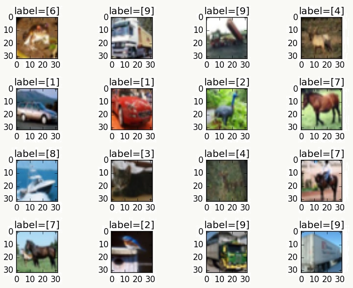
def data_visualize(x, y, num):
plt.figure()
for i in range(0, num * num):
axes = plt.subplot(num, num, i + 1)
axes.set_title("label=" + str(y[i]))
axes.set_xticks([0, 10, 20, 30])
axes.set_yticks([0, 10, 20, 30])
plt.imshow(toimage(x[i]))
plt.tight_layout()
plt.savefig('sample.jpg')
if __name__ == "__main__":
from keras.utils.vis_utils import plot_model
with tf.device('/gpu:3'):
gpu_options = tf.GPUOptions(per_process_gpu_memory_fraction=1, allow_growth=True)
os.environ["CUDA_VISIBLE_DEVICES"] = "3"
tf.Session(config=K.tf.ConfigProto(allow_soft_placement=True,
log_device_placement=True,
gpu_options=gpu_options))
(X_train, y_train), (X_test, y_test) = cifar10.load_data()
data_visualize(X_train, y_train, 4)
# 定义输入数据并做归一化
dim = 32
channel = 3
class_num = 10
X_train = X_train.reshape(X_train.shape[0], dim, dim, channel).astype('float32') / 255
X_test = X_test.reshape(X_test.shape[0], dim, dim, channel).astype('float32') / 255
Y_train = np_utils.to_categorical(y_train, class_num)
Y_test = np_utils.to_categorical(y_test, class_num)
# this will do preprocessing and realtime data augmentation
datagen = ImageDataGenerator(
featurewise_center=False, # set input mean to 0 over the dataset
samplewise_center=False, # set each sample mean to 0
featurewise_std_normalization=False, # divide inputs by std of the dataset
samplewise_std_normalization=False, # divide each input by its std
zca_whitening=False, # apply ZCA whitening
rotation_range=25, # randomly rotate images in the range (degrees, 0 to 180)
width_shift_range=0.1, # randomly shift images horizontally (fraction of total width)
height_shift_range=0.1, # randomly shift images vertically (fraction of total height)
horizontal_flip=True, # randomly flip images
vertical_flip=False) # randomly flip images
datagen.fit(X_train)
s = X_train.shape[1:]
print(s)
builder = resnet.ResNet("ResNet-test")
resnet_34 = builder.residual_builder(s, class_num, builder.basic_block, [3, 4, 6, 3])
model = resnet_34
model.summary()
#import pdb
#pdb.set_trace()
plot_model(model, to_file="ResNet.jpg", show_shapes=True)
model.compile(loss='categorical_crossentropy',
optimizer='adadelta',
metrics=['accuracy'])
batch_size = 32
nb_epoch = 100
# import pdb
# pdb.set_trace()
ModelCheckpoint("weights-improvement-{epoch:02d}-{val_acc:.2f}.hdf5", monitor='val_loss', verbose=0,
save_best_only=False, save_weights_only=False, mode='auto')
model.fit_generator(datagen.flow(X_train, Y_train, batch_size=batch_size),
steps_per_epoch=X_train.shape[0],
validation_data=(X_test, Y_test),
epochs=nb_epoch,
verbose=1,
max_q_size=100,
callbacks=[lr_reducer, early_stopper, csv_logger])
score = model.evaluate(X_test, Y_test, verbose=0)
print('Test score:', score[0])
print('Test accuracy:', score[1])graphviz安装 yum list available 'graphviz' yum install 'graphviz'
pydot_ng安装 pip install pydot_ng
网络结构
![]()
可以看到网络结构很复杂但需要训练的参数个数只有21296522个,远小于AlexNet参数个数。
- CIFAR-10训练情况
![]()
迭代100次后,训练集上Acc为:0.8367,测试集上Acc为0.8346。
5.10 Maxout Networks
Goodfellow等人在《Maxout Networks》一文中提出,这篇论文值得一看。 ### 5.10.1 Maxout激活函数 对于神经网络任意一层可以添加Maxout结构,公式如下: \[ \begin{array}{l} h_i(x)=max_{j\in [1,k]}z_{ij}\\ z_{ij}=x^TW_{...ij}+b_{ij} \end{array} \] 上面的\(W\)和\(b\)是要学习的参数,这些参数可以通过反向传播计算,\(k\)是事先指定的参数,\(x\)是输入节点,假定有以下3层网络结构:
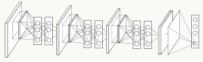
Maxout激活可以认为是在输入节点\(x\)和输出节点\(h\)中间加了\(k\)个隐含节点,以上图节点\(i\)为例,上图红色部分在Maxout结构中被扩展为以下结构:
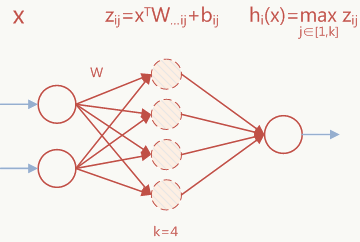
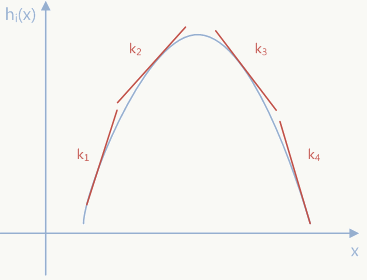
从全局上看,ReLU可以看做Maxout的一种特例,Maxout通过网络自动学习激活函数(从这个角度看Maxout也可以看做某种Network-In-Network结构),不对\(k\)做限制,只要两个Maxout 单元就能拟合任意连续函数,关于这部分论文中有更详细的证明,这里不再赘述,实际上它与Dropout配合效果更好,这里可以回想下核方法(Kernel Method),核方法采用非线性核(如高斯核)也会有类似通过局部线性拟合来模拟非线性行为,但传统核方法会事先指定核函数(如高斯函数),而不是数据驱动的方式算出来,当然也有kernel组合方面的研究,但在我看来最终和神经网络殊途同归,其实都可以在神经网络的大框架下去思考(回想前面的SVM与神经网络的关系)。 凡事都有两面性,Maxout的缺点也是明显的:多了一倍参数、需要人为指定\(k\)值、先验假设被学习的激活函数是凸的。
5.11 Network in Network
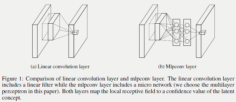
NIN的思想来源于《Network In Network》,其亮点有2个方面:将传统卷积层替换为非线性卷积层以提升特征抽象能力;使用新的pooling层代替传统全连接层,后续出现的各个版本GoogLeNet也很大程度借鉴了这个思想。
5.11.1 NIN卷积层(MLP Convolution)
传统卷积操作,例如:\(f_{i,j,k}=max(W_k^T \cdot x_{i,j},0)\),本质是广义线性模型,意味着当数据接近线性可分时模型效果会比较好,反之亦然。Maxout网络在一定程度上解决了这个问题,但它有凸函数的假设,实际当中可能很多情况是非凸的,所以论文提出使用多层感知机(MLP)来拟合,不做任何先验假设。 选择MLP的原因是:
MLP能拟合任意函数,不需要做先验假设(如:线性可分、凸集);
MLP与卷积神经网络结构天然兼容,可以通过BP方便的做训练;
MLP本身也能做的较深,且特征能够得到复用;
通过MLP做卷积可以起到feature map级联交叉加权组合的作用,能提升特征抽象能力: \[ \begin{array}{l} f^1_{i,j,k_1}=max({w^1_{k_1}}^Tx_{i,j}+b_{k_1},0)\\ \quad\quad \quad .\\ \quad\quad \quad .\\ \quad\quad \quad .\\ f^1_{i,j,k_n}=max({w^n_{k_n}}^Tf_{i,j}^{n-1}+b_{k_n},0). \end{array} \]
![]()
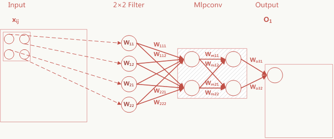
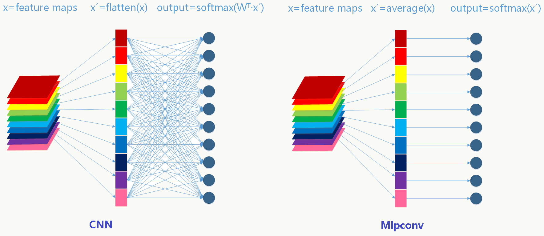
\[ \begin{array}{l} O_1=\sum_{i=1}^2\sum_{j=1}^2x_{ij} \cdot W_{ij} \cdot (C_1 \cdot W_{1ij}+ C_2 \cdot W_{ij,2})\\ C1=W_{m11}W_{o31}+W_{m12}W_{o32}\\ C2=W_{m21}W_{o31}+W_{m22}W_{o32} \end{array} \] \(O_1\)的前半部分是传统卷积层,后半部分可以看做1×1卷积层。 ### 5.11.2 NIN抽样层(Global Average Pooling) 把传统卷积网络分两部分看待:除全连接层外的各个卷积层看做特征提取器,全连接层看成特征组合器。由于全连接的存在破坏了数据的可解释性并大大增加了可训练参数的个数,NIN通过GAP来避免这两个问题,具体做法是:
- 最后一层卷积feature map的个数与分类类别数一致,这种一致性可以产生相对较少的feature map,比如有10个分类和10个n×n的feature map;
- 每个feature map对应一个分类,并对整个feature map求平均值,这种方法能提高空间变换的稳定性,但损失了位置信息(例如在目标检测中位置信息很重要),比如10个n×n的feature map会得到10个实数值组成的一维向量;
- 用softmax做归一化,注意这里要区分传统CNN下的softmax激活和softmax归一,这一层没有需要优化的参数。 传统CNN与Mlpconv的区别如下图:
![]()
5.12 GoogLeNet Inception V1
GoogLeNet是由google的Christian Szegedy等人在2014年的论文《Going Deeper with Convolutions》提出,其最大的亮点是提出一种叫Inception的结构,以此为基础构建GoogLeNet,并在当年的ImageNet分类和检测任务中获得第一,ps:GoogLeNet的取名是为了向YannLeCun的LeNet系列致敬。
5.12.1 一些思考
为了提高深度神经网络的性能,最简单粗暴有效的方法是增加网络深度与宽度,但这个方法有两个明显的缺点:
- 更深更宽的网络意味着更多的参数,从而大大增加过拟合的风险,尤其在训练数据不是那么多或者某个label训练数据不足的情况下更容易发生;
- 增加计算资源的消耗,实际情况下,不管是因为数据稀疏还是扩充的网络结构利用不充分(比如很多权重接近0),都会导致大量计算的浪费。
解决以上两个问题的基本方法是将全连接或卷积连接改为稀疏连接。不管从生物的角度还是机器学习的角度,稀疏性都有良好的表现,回想Dropout网络以及ReLU激活函数,其本质就是利用稀疏性提高模型泛化性(但需要计算的参数没变少)。 简单解释下稀疏性,当整个特征空间是非线性甚至不连续时:
- 学好局部空间的特征集更能提升性能,类似于Maxout网络中使用多个局部线性函数的组合来拟合非线性函数的思想;
- 假设整个特征空间由N个不连续局部特征空间集合组成,任意一个样本会被映射到这N个空间中并激活/不激活相应特征维度,如果用C1表示某类样本被激活的特征维度集合,用C2表示另一类样本的特征维度集合,当数据量不够大时,要想增加特征区分度并很好的区分两类样本,就要降低C1和C2的重合度(比如可用Jaccard距离衡量),即缩小C1和C2的大小,意味着相应的特征维度集会变稀疏。
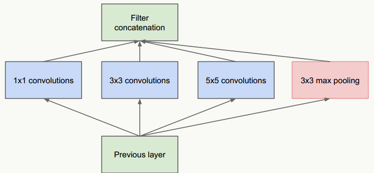
- 把不同大小卷积核抽象得到的特征空间看做子特征空间,每个子特征空间都是稀疏的,把这些不同尺度特征做融合,相当于得到一个相对稠密的空间;
- 采用1×1、3×3、5×5卷积核(不是必须的,也可以是其他大小),stride取1,利用padding可以方便的做输出特征维度对齐;
- 大量事实表明pooling层能有效提高卷积网络的效果,所以加了一条max pooling路径;
- 这个结构符合直观理解,视觉信息通过不同尺度的变换被聚合起来作为下一阶段的特征,比如:人的高矮、胖瘦、青老信息被聚合后做下一步判断。
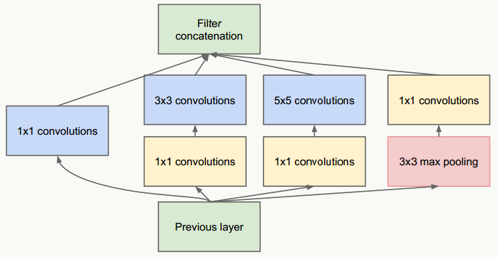
这个网络的最大问题是5×5卷积带来了巨大计算负担,例如,假设上层输入为:28×28×192:
- 直接经过96个5×5卷积层(stride=1,padding=2)后,输出为:28×28×96,卷积层参数量为:192×5×5×96=460800;
- 借鉴NIN网络,在5×5卷积前使用32个1×1卷积核做维度缩减,变成28×28×32,之后经过96个5×5卷积层(stride=1,padding=2)后,输出为:28×28×96,但所有卷积层的参数量为:192×1×1×32+32×5×5×96=82944,可见整个参数量是原来的1/5.5,且效果上没有多少损失。 新网络结构为:
![]()
5.12.2 GoogLeNet结构
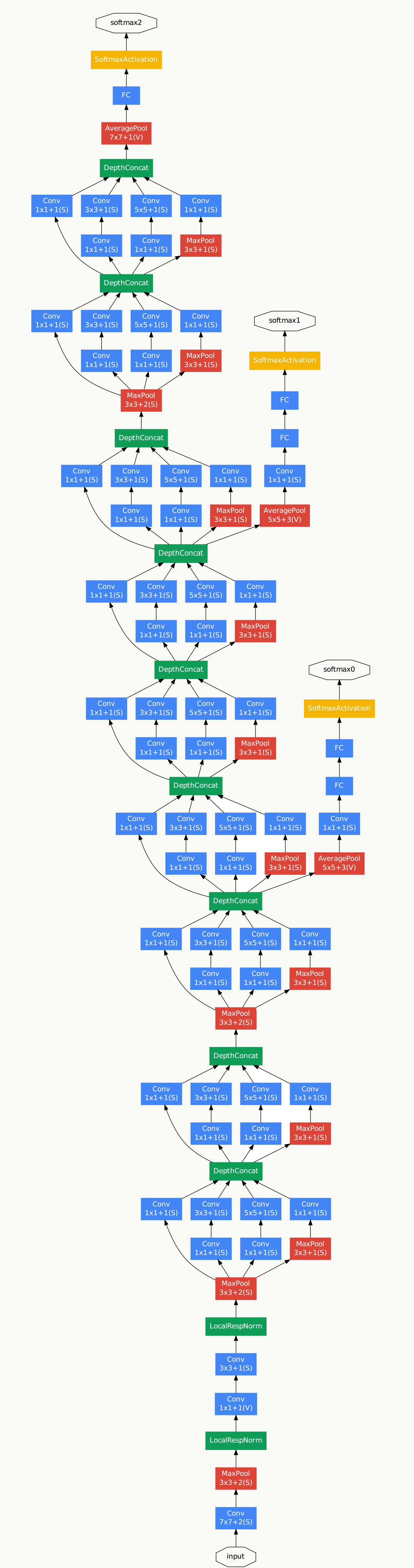
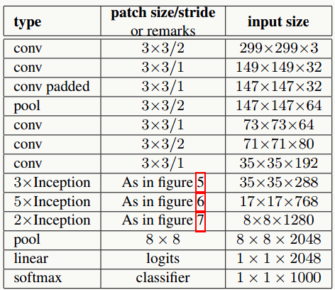
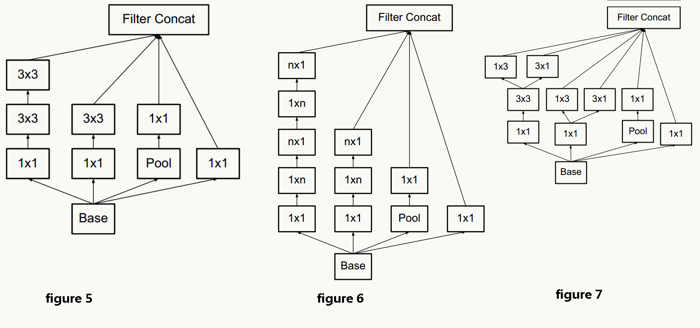
利用上述Inception模块构建GoogLeNet,实验表明Inception模块出现在高层特征抽象时会更加有效(我理解由于其结构特点,更适合提取高阶特征,让它提取低阶特征会导致特征信息丢失),所以在低层依然使用传统卷积层。整个网路结构如下: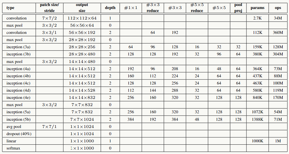
网络说明:
- 所有卷积层均使用ReLU激活函数,包括做了1×1卷积降维后的激活;
- 移除全连接层,像NIN一样使用Global Average Pooling,使得Top 1准确率提高0.6%,但由于GAP与类别数目有关系,为了方便大家做模型fine-tuning,最后加了一个全连接层;
- 与前面的ResNet类似,实验观察到,相对浅层的神经网络层对模型效果有较大的贡献,训练阶段通过对Inception(4a、4d)增加两个额外的分类器来增强反向传播时的梯度信号,但最重要的还是正则化作用,这一点在GoogLeNet v3中得到实验证实,并间接证实了GoogLeNet V2中BN的正则化作用,这两个分类器的loss会以0.3的权重加在整体loss上,在模型inference阶段,这两个分类器会被去掉;
- 用于降维的1×1卷积核个数为128个;
- 全连接层使用1024个神经元;
- 使用丢弃概率为0.7的Dropout层;
网络结构说明:
输入数据为224×224×3的RGB图像,图中"S"代表做same-padding,"V"代表不做。
- C1卷积层:64个7×7卷积核(stride=2,padding=3),输出为:112×112×64;
- P1抽样层:64个3×3卷积核(stride=2),输出为56×56×64,其中:56=(112-3+1)/2+1
- C2卷积层:192个3×3卷积核(stride=1,padding=1),输出为:56×56×192;
- P2抽样层:192个3×3卷积核(stride=2),输出为28×28×192,其中:28=(56-3+1)/2+1,接着数据被分出4个分支,进入Inception (3a)
- Inception (3a):由4部分组成
- 64个1×1的卷积核,输出为28×28×64;
- 96个1×1的卷积核做降维,输出为28×28×96,之后128个3×3卷积核(stride=1,padding=1),输出为:28×28×128
- 16个1×1的卷积核做降维,输出为28×28×16,之后32个5×5卷积核(stride=1,padding=2),输出为:28×28×32
- 192个3×3卷积核(stride=1,padding=1),输出为28×28×192,进行32个1×1卷积核,输出为:28×28×32 最后对4个分支的输出做“深度”方向组合,得到输出28×28×256,接着数据被分出4个分支,进入Inception (3b);
- Inception (3b):由4部分组成
- 128个1×1的卷积核,输出为28×28×128;
- 128个1×1的卷积核做降维,输出为28×28×128,进行192个3×3卷积核(stride=1,padding=1),输出为:28×28×192
- 32个1×1的卷积核做降维,输出为28×28×32,进行96个5×5卷积核(stride=1,padding=2),输出为:28×28×96
- 256个3×3卷积核(stride=1,padding=1),输出为28×28×256,进行64个1×1卷积核,输出为:28×28×64 最后对4个分支的输出做“深度”方向组合,得到输出28×28×480; 后面结构以此类推。
5.12.3 代码实践
googlenet_inception_v1.py
1
2
3
4
5
6
7
8
9
10
11
12
13
14
15
16
17
18
19
20
21
22
23
24
25
26
27
28
29
30
31
32
33
34
35
36
37
38
39
40
41
42
43
44
45
46
47
48
49
50
51
52
53
54
55
56
57
58
59
60
61
62
63
64
65
66
67
68
69
70
71
72
73
74
75
76
77
78
79
80
81
82
83
84
85
86
87
88
89
90
91
92
93
94
95
96
97
98
99
100
101
102
103
104
105
106
107
108
109
110
111
112
113
114
115
116
117
118
119
120
121
122
123
124
125
126
127
128
129
130
131
132
133
134
135
136
137
138
139
140
141
142
143
144
145
146
147
148
149
150
151
152
153
154
155
156
157
158
159
160
161
162
163
164
165
166
167
168
169
170
171
172
173
174
175
176
177
178
179
180
181
182
183
184
185
186
187
188
189
190
191
192
193
194
195
196
197
198
199
200
201
202
203
204
205
206
207
208
209
210
211
212
213
214
215
216
217
218
219
220
221
222
223
224
225
226
227
228
229
230
231
232
233
234
235
236
237
238
239
240
241
242
243
244
245
246
247
248
249
250
251
252
253
254
255
256
257
258
259
260
261# -*- coding: utf-8 -*-
from keras.layers import Input, Conv2D, Dense, MaxPooling2D, AveragePooling2D
from keras.layers import Dropout, Flatten, merge, ZeroPadding2D, Reshape, Activation
from keras.models import Model
from keras.regularizers import l1_l2
import tensorflow as tf
import googlenet_custom_layers
def inception_module(name,
input_layer,
num_c_1x1,
num_c_1x1_3x3_reduce,
num_c_3x3,
num_c_1x1_5x5_reduce,
num_p_5x5,
num_c_1x1_reduce):
inception_1x1 = Conv2D(name=name+"/inception_1x1",
filters=num_c_1x1,
kernel_size=(1, 1),
strides=(1, 1),
padding='same',
kernel_initializer='he_normal',
activation='relu',
kernel_regularizer=l1_l2(0.0001))(input_layer)
inception_3x3_reduce = Conv2D(name=name+"/inception_3x3_reduce",
filters=num_c_1x1_3x3_reduce,
kernel_size=(1, 1),
strides=(1, 1),
padding='same',
kernel_initializer='he_normal',
activation='relu',
kernel_regularizer=l1_l2(0.0001))(input_layer)
inception_3x3 = Conv2D(name=name+"/inception_3x3",
filters=num_c_3x3,
kernel_size=(3, 3),
strides=(1, 1),
padding='same',
kernel_initializer='he_normal',
activation='relu',
kernel_regularizer=l1_l2(0.0001))(inception_3x3_reduce)
inception_5x5_reduce = Conv2D(name=name+"/inception_5x5_reduce",
filters=num_c_1x1_5x5_reduce,
kernel_size=(1, 1),
strides=(1, 1),
padding='same',
kernel_initializer='he_normal',
activation='relu',
kernel_regularizer=l1_l2(0.0001))(input_layer)
inception_5x5 = Conv2D(name=name+"/inception_5x5",
filters=num_p_5x5,
kernel_size=(5, 5),
strides=(1, 1),
padding='same',
kernel_initializer='he_normal',
activation='relu',
kernel_regularizer=l1_l2(0.0001))(inception_5x5_reduce)
inception_max_pool = MaxPooling2D(name=name+"/inception_max_pool",
pool_size=(3, 3),
strides=(1, 1),
padding="same")(input_layer)
inception_max_pool_proj = Conv2D(name=name+"/inception_max_pool_project",
filters=num_c_1x1_reduce,
kernel_size=(1, 1),
strides=(1, 1),
padding='same',
kernel_initializer='he_normal',
activation='relu',
kernel_regularizer=l1_l2(0.0001))(inception_max_pool)
print (inception_1x1.get_shape(), inception_3x3.get_shape(), inception_5x5.get_shape(), inception_max_pool_proj.get_shape())
# inception_output = tf.concat(3, [inception_1x1, inception_3x3, inception_5x5, inception_max_pool_proj])
from keras.layers.merge import concatenate
#注意,由于变态的tensorflow更改了concat函数的参数顺序,需要注意自己的tf和keras版本
#适时的将/usr/lib/python×××/site-packages/keras/backend/tensorflow_backend.py的1554行的代码由
#return tf.concat([to_dense(x) for x in tensors], axis) 改为:
#return tf.concat(axis, [to_dense(x) for x in tensors])
inception_output = concatenate([inception_1x1, inception_3x3, inception_5x5, inception_max_pool_proj])
return inception_output
def googLeNet_inception_v1_building(input_shape, output_num, fine_tune=None):
input_layer = Input(shape=input_shape)
# 第一层,卷积层
conv1_7x7 = Conv2D(name="conv1_7x7/2",
filters=64,
kernel_size=(7, 7),
strides=(2, 2),
padding='same',
kernel_initializer='he_normal',
activation='relu',
kernel_regularizer=l1_l2(0.0001))(input_layer)
conv1_zero_pad = ZeroPadding2D(padding=(1, 1))(conv1_7x7)
# 第二层,max pooling层
pool1_3x3 = MaxPooling2D(name="max_pool1_3x3/2",
pool_size=(3, 3),
strides=(2, 2),
padding='valid')(conv1_zero_pad)
# 第二层,LRN规范化
#pool1_norm1 = tf.nn.lrn(pool1_3x3, 4, bias=1.0, alpha=0.001 / 9.0, beta=0.75, name='ax_pool1_3x3/norm1')
pool1_norm1 = googlenet_custom_layers.LRN2D(name='max_pool1_3x3/norm1')(pool1_3x3)
# 第四层,卷积层降维
conv2_3x3_reduce = Conv2D(name="conv2_3x3_reduce/1",
filters=64,
kernel_size=(1, 1),
padding='same',
kernel_initializer='he_normal',
activation='relu',
kernel_regularizer=l1_l2(0.0001))(pool1_norm1)
# 第五层,卷积层
conv2_3x3 = Conv2D(name="conv2_3x3/1",
filters=192,
kernel_size=(3, 3),
padding='same',
kernel_initializer='he_normal',
activation='relu',
kernel_regularizer=l1_l2(0.0001))(conv2_3x3_reduce)
# 第六层,LRN规范化
#conv2_norm2 = tf.nn.lrn(conv2_3x3, 4, bias=1.0, alpha=0.001 / 9.0, beta=0.75, name='conv2_3x3/norm2')
conv2_norm2 = googlenet_custom_layers.LRN2D(name='conv2_3x3/norm2')(conv2_3x3)
conv2_zero_pad = ZeroPadding2D(padding=(1, 1))(conv2_norm2)
# 第七层,max pooling层
pool2_3x3 = MaxPooling2D(name="max_pool2_3x3",
pool_size=(3, 3),
strides=(2, 2),
padding='valid')(conv2_zero_pad)
# 第八层,inception 3a
inception_3a = inception_module("inception_3a",pool2_3x3, 64, 96, 128, 16, 32, 32)
# 第九层,inception 3b
inception_3b = inception_module("inception_3b",inception_3a, 128, 128, 192, 32, 96, 64)
inception_3b_zero_pad = ZeroPadding2D(padding=(1, 1))(inception_3b)
# 第十层,max pooling层
pool3_3x3 = MaxPooling2D(name="max_pool3_3x3/2",
pool_size=(3, 3),
strides=(2, 2),
padding='valid')(inception_3b_zero_pad)
# 第十一层,inception 4a
inception_4a = inception_module("inception_4a",pool3_3x3, 192, 96, 208, 16, 48, 64)
# 第十二层,分支loss1
loss1_ave_pool = AveragePooling2D(name="loss1/ave_pool",
pool_size=(5, 5),
strides=(3, 3))(inception_4a)
loss1_conv = Conv2D(name="loss1/conv",
filters=128,
kernel_size=(1, 1),
padding='same',
kernel_initializer='he_normal',
activation='relu',
kernel_regularizer=l1_l2(0.0001))(loss1_ave_pool)
loss1_flat = Flatten()(loss1_conv)
loss1_fc = Dense(1024,
activation='relu',
name="loss1/fc",
kernel_regularizer=l1_l2(0.0001))(loss1_flat)
loss1_drop_fc = Dropout(0.7)(loss1_fc)
loss1_classifier = Dense(output_num,
name="loss1/classifier",
kernel_regularizer=l1_l2(0.0001))(loss1_drop_fc)
loss1_classifier_act = Activation('softmax')(loss1_classifier)
# 第十二层,inception_4b
inception_4b = inception_module("inception_4b",inception_4a, 160, 112, 224, 24, 64, 64)
# 第十三层,inception_4c
inception_4c = inception_module("inception_4c",inception_4b, 128, 128, 256, 24, 64, 64)
# 第十四层,inception_4c
inception_4d = inception_module("inception_4d",inception_4c, 112, 144, 288, 32, 64, 64)
# 第十五层,分支loss2
loss2_ave_pool = AveragePooling2D(pool_size=(5, 5),
strides=(3, 3),
name='loss2/ave_pool')(inception_4d)
loss2_conv = Conv2D(name="loss2/conv",
filters=128,
kernel_size=(1, 1),
padding='same',
kernel_initializer='he_normal',
activation='relu',
kernel_regularizer=l1_l2(0.0001))(loss2_ave_pool)
loss2_flat = Flatten()(loss2_conv)
loss2_fc = Dense(1024,
activation='relu',
name="loss2/fc",
kernel_regularizer=l1_l2(0.0001))(loss2_flat)
loss2_drop_fc = Dropout(0.7)(loss2_fc)
loss2_classifier = Dense(output_num,
name="loss2/classifier",
kernel_regularizer=l1_l2(0.0001))(loss2_drop_fc)
loss2_classifier_act = Activation('softmax')(loss2_classifier)
# 第十五层,inception_4e
inception_4e = inception_module("inception_4e",inception_4d, 256, 160, 320, 32, 128, 128)
inception_4e_zero_pad = ZeroPadding2D(padding=(1, 1))(inception_4e)
# 第十六层,max pooling层
pool4_3x3 = MaxPooling2D(name="max_pool4_3x3",
pool_size=(3, 3),
strides=(2, 2),
padding='valid')(inception_4e_zero_pad)
# 第十七层,inception_5a
inception_5a = inception_module("inception_5a",pool4_3x3, 256, 160, 320, 32, 128, 128)
# 第十八层,inception_5b
inception_5b = inception_module("inception_5b",inception_5a, 384, 192, 384, 48, 128, 128)
# 第十九层,average pooling层
pool5_7x7 = AveragePooling2D(name="ave_pool5_7x7",
pool_size=(7, 7),
strides=(1, 1))(inception_5b)
loss3_flat = Flatten()(pool5_7x7)
pool5_drop_7x7 = Dropout(0.4)(loss3_flat)
# 第二十层,全连接层
loss3_classifier = Dense(output_num,
name="loss3/classifier",
kernel_regularizer=l1_l2(0.0001))(pool5_drop_7x7)
loss3_classifier_act = Activation('softmax')(loss3_classifier)
googlenet_inception_v1 = Model(name="googlenet_inception_v1",
input=input_layer,
output=[loss1_classifier_act, loss2_classifier_act, loss3_classifier_act])
if fine_tune:
googlenet_inception_v1.load_weights(fine_tune)
return googlenet_inception_v1googlenet_custom_layers.py
1
2
3
4
5
6
7
8
9
10
11
12
13
14
15
16
17
18
19
20
21
22
23
24
25
26
27
28
29
30
31
32
33
34
35
36
37
38
39
40
41
42
43
44
45
46
47
48
49
50
51
52
53
54
55
from keras.layers.core import Layer
import keras.backend as K
class LRN2D(Layer):
"""
This code is adapted from pylearn2.
License at: https://github.com/lisa-lab/pylearn2/blob/master/LICENSE.txt
"""
def __init__(self, alpha=1e-4, k=2, beta=0.75, n=5, **kwargs):
if n % 2 == 0:
raise NotImplementedError("LRN2D only works with odd n. n provided: " + str(n))
super(LRN2D, self).__init__(**kwargs)
self.alpha = alpha
self.k = k
self.beta = beta
self.n = n
def get_output(self, train):
X = self.get_input(train)
b, ch, r, c = K.shape(X)
half_n = self.n // 2
input_sqr = K.square(X)
extra_channels = K.zeros((b, ch + 2 * half_n, r, c))
input_sqr = K.concatenate([extra_channels[:, :half_n, :, :],
input_sqr,
extra_channels[:, half_n + ch:, :, :]],
axis=1)
scale = self.k
for i in range(self.n):
scale += self.alpha * input_sqr[:, i:i + ch, :, :]
scale = scale ** self.beta
return X / scale
def get_config(self):
config = {"name": self.__class__.__name__,
"alpha": self.alpha,
"k": self.k,
"beta": self.beta,
"n": self.n}
base_config = super(LRN2D, self).get_config()
return dict(list(base_config.items()) + list(config.items()))
class PoolHelper(Layer):
def __init__(self, **kwargs):
super(PoolHelper, self).__init__(**kwargs)
def call(self, x, mask=None):
return x[:, :, 1:, 1:]
def get_config(self):
config = {}
base_config = super(PoolHelper, self).get_config()
return dict(list(base_config.items()) + list(config.items()))googlenet_inception_v1-cifar10.py
1
2
3
4
5
6
7
8
9
10
11
12
13
14
15
16
17
18
19
20
21
22
23
24
25
26
27
28
29
30
31
32
33
34
35
36
37
38
39
40
41
42
43
44
45
46
47
48
49
50
51
52
53
54
55
56
57
58
59
60
61
62
63
64
65
66
67
68
69
70
71
72
73
74
75
76
77
78
79
80
81
82
83
84
85
86
87
88
89
90
91
92
93
# -*- coding: utf-8 -*-
import numpy as np
import matplotlib
matplotlib.use("Agg")
import matplotlib.pyplot as plt
import os
from scipy.misc import toimage
from keras.datasets import cifar10
from keras.utils import np_utils
from keras.preprocessing.image import ImageDataGenerator
from keras.callbacks import ModelCheckpoint
from keras import backend as K
import tensorflow as tf
tf.python.control_flow_ops = tf
from keras.callbacks import ReduceLROnPlateau, CSVLogger, EarlyStopping
lr_reducer = ReduceLROnPlateau(monitor='val_loss', factor=np.sqrt(0.5), cooldown=0, patience=3, min_lr=1e-6)
early_stopper = EarlyStopping(monitor='val_acc', min_delta=0.0005, patience=15)
csv_logger = CSVLogger('resnet34_cifar10.csv')
import os
import googlenet_inception_v1
if __name__ == "__main__":
from keras.utils.vis_utils import plot_model
with tf.device('/gpu:4'):
gpu_options = tf.GPUOptions(per_process_gpu_memory_fraction=1, allow_growth=True)
os.environ["CUDA_VISIBLE_DEVICES"] = "4"
tf.Session(config=K.tf.ConfigProto(allow_soft_placement=True,
log_device_placement=True,
gpu_options=gpu_options))
(X_train, y_train), (X_test, y_test) = cifar10.load_data()
# 定义输入数据并做归一化
dim = 32
channel = 3
class_num = 10
X_train = X_train.reshape(X_train.shape[0], dim, dim, channel).astype('float32') / 255
X_test = X_test.reshape(X_test.shape[0], dim, dim, channel).astype('float32') / 255
Y_train = np_utils.to_categorical(y_train, class_num)
Y_test = np_utils.to_categorical(y_test, class_num)
# this will do preprocessing and realtime data augmentation
datagen = ImageDataGenerator(
featurewise_center=False, # set input mean to 0 over the dataset
samplewise_center=False, # set each sample mean to 0
featurewise_std_normalization=False, # divide inputs by std of the dataset
samplewise_std_normalization=False, # divide each input by its std
zca_whitening=False, # apply ZCA whitening
rotation_range=25, # randomly rotate images in the range (degrees, 0 to 180)
width_shift_range=0.1, # randomly shift images horizontally (fraction of total width)
height_shift_range=0.1, # randomly shift images vertically (fraction of total height)
horizontal_flip=True, # randomly flip images
vertical_flip=False) # randomly flip images
datagen.fit(X_train)
s = X_train.shape[1:]
print(s)
model = googlenet_inception_v1.googLeNet_inception_v1_building(s,class_num)
model.summary()
#import pdb
#pdb.set_trace()
plot_model(model, to_file="GoogLeNet-Inception-V1.jpg", show_shapes=True)
model.compile(loss='categorical_crossentropy',
optimizer='adadelta',
metrics=['accuracy'])
batch_size = 32
nb_epoch = 100
# import pdb
# pdb.set_trace()
ModelCheckpoint("weights-improvement-{epoch:02d}-{val_acc:.2f}.hdf5", monitor='val_loss', verbose=0,
save_best_only=False, save_weights_only=False, mode='auto')
for e in range(nb_epoch):
batches = 0
for X_batch, Y_batch in datagen.flow(X_train, Y_train, batch_size=64):
loss = model.train_on_batch(X_batch, [Y_batch,Y_batch,Y_batch]) # note the three outputs
print loss
#print '\r\n'
#loss_and_metrics = model.evaluate(X_test, [Y_test,Y_test,Y_test], batch_size=128)
#model.fit(X_test, [Y_test,Y_test,Y_test], batch_size=64)
batches += 1
if batches >= len(X_train) / 64:
# we need to break the loop by hand because
# the generator loops indefinitely
break
score = model.evaluate(X_test, Y_test, verbose=0)
print('Test score:', score[0])
print('Test accuracy:', score[1])
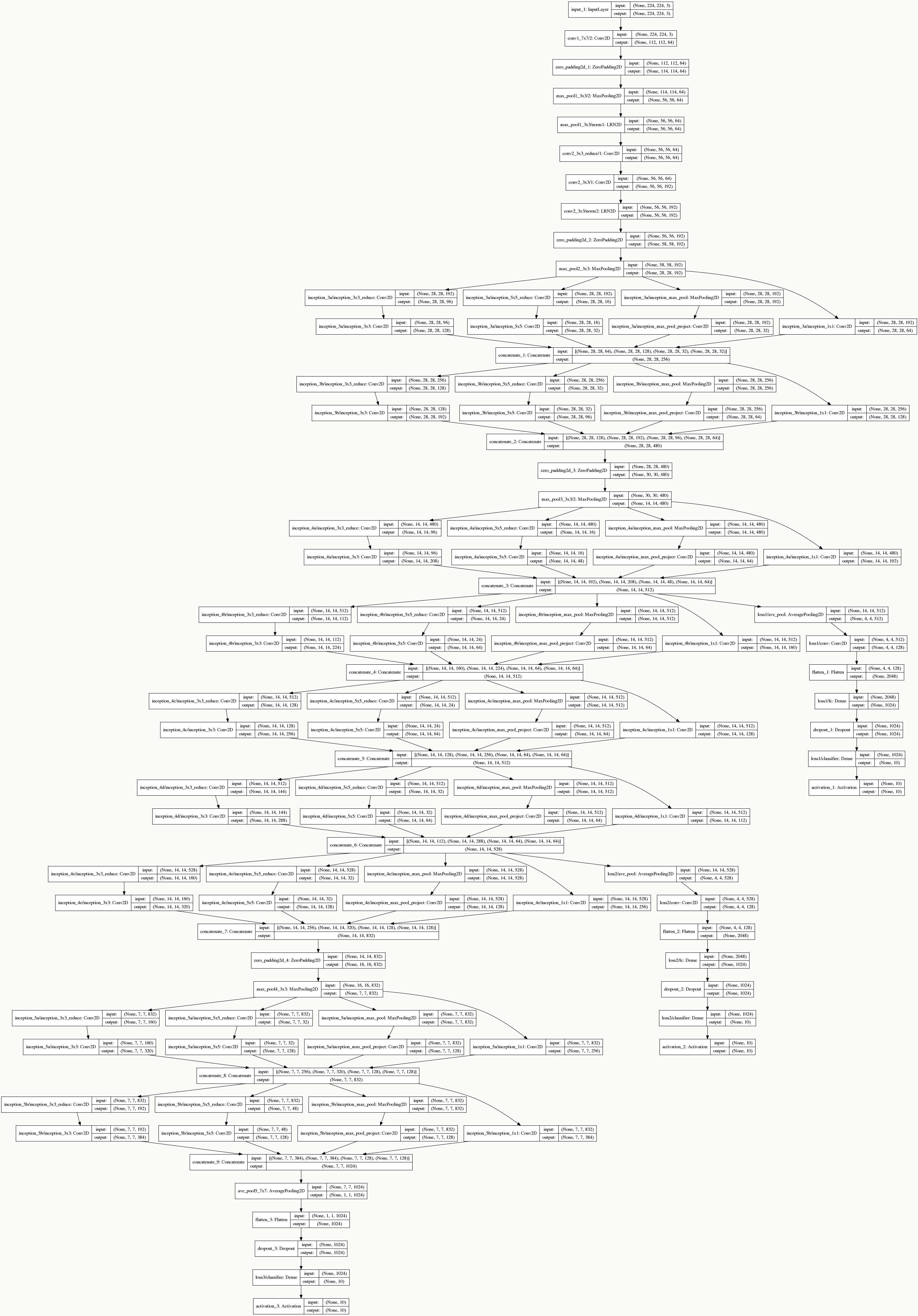
需要训练的总参数量为10,334,030个。
5.13 GoogLeNet Inception V2
GoogLeNet Inception V2在《Batch Normalization: Accelerating Deep Network Training by Reducing Internal Covariate Shift》出现,最大亮点是提出了Batch Normalization方法,它起到以下作用:
- 使用较大的学习率而不用特别关心诸如梯度爆炸或消失等优化问题;
- 降低了模型效果对初始权重的依赖;
- 可以加速收敛,一定程度上可以不使用Dropout这种降低收敛速度的方法,但却起到了正则化作用提高了模型泛化性;
- 即使不使用ReLU也能缓解激活函数饱和问题;
- 能够学习到从当前层到下一层的分布缩放( scaling (方差),shift (期望))系数。
5.13.1 一些思考
在机器学习中,我们通常会做一种假设:训练样本独立同分布(iid)且训练样本与测试样本分布一致,如果真实数据符合这个假设则模型效果可能会不错,反之亦然,这个在学术上叫Covariate Shift,所以从样本(外部)的角度说,对于神经网络也是一样的道理。从结构(内部)的角度说,由于神经网络由多层组成,样本在层与层之间边提特征边往前传播,如果每层的输入分布不一致,那么势必造成要么模型效果不好,要么学习速度较慢,学术上这个叫Internal Covariate Shift。
假设:\(y\)为样本标注,\(X=\{x_1,x_2,x_3,......\}\)为样本\(x\)通过神经网络若干层后每层的输入;
理论上:\(p(x,y)\)的联合概率分布应该与集合\(X\)中任意一层输入的联合概率分布一致,如:\(p(x,y)=p(x_1,y)\); 但是:\(p(x,y)=p(y|x) \cdot p(x)\),其中条件概率\(p(y|x)\)是一致的,即\(p(y|x)=p(y|x_1)=p(y|x_2)=......\),但由于神经网络每一层对输入分布的改变,导致边缘概率是不一致的,即\(p(x)\neq p(x_1)\neq p(x_2)......\),甚至随着网络深度的加深,前面层微小的变化会导致后面层巨大的变化。
5.13.2 BN原理
BN整个算法过程如下:
\[ \begin{align*} & \text{Input: Values of $x$ over a mini-batch: $B=\{x_1...m\}$} \\ & \text{ $\qquad \quad$ Paramters to be learned:$\gamma$,$\beta$} \\ & \text{Output:} \{y_i = BN_{\gamma,\beta}(x_i)\} \\ & \quad \mu_{B} \gets \frac{1}{m} \sum_{i=1}^{m}{x_i} \qquad &&\text{//mini-batch mean}\\ & \quad \sigma^2_B \gets \frac{1}{m} \sum_{i=1}^{m}{(x_i-\mu_B)^2} \qquad &&\text{//mini-batch variance}\\ & \quad \hat{x}_i \gets \frac{x_i-\mu_B}{\sqrt{\sigma_B^2 +\epsilon}} \qquad &&\text{//normalize}\\ & \quad y_i \gets \gamma\hat{x}_i+\beta \equiv BN_{\gamma,\beta}(x_i) \qquad &&\text{//scale and shift}\\ \end{align*} \]
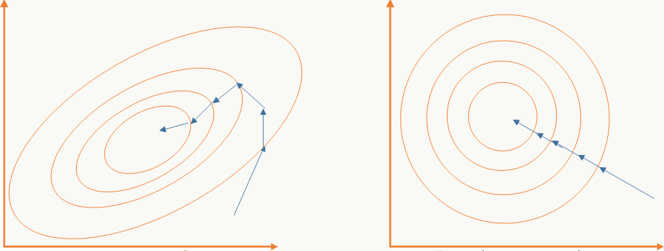
- 以batch的方式做训练,对m个样本求期望和方差后对训练数据做白化,通过白化操作可以去除特征相关性并把数据缩放在一个球体上,这么做的好处既可以加快优化算法的优化速度也可能提高优化精度,一个直观的解释:
![]()
- 当原始输入对模型学习更有利时能够恢复原始输入(和残差网络有点神似):
![]()
这里的参数\(\gamma\)和\(\sigma\)是需要学习的。
参数学习依然是利用反向传播原理:
\[ \begin{align*} & \frac{\partial l}{\partial \hat{x}_i}=\frac{\partial l}{\partial \hat{y}_i} \cdot \gamma \\ & \frac{\partial l}{\partial \sigma_B^2}=\sum_{i=1}^{m}\frac{\partial l}{\partial \hat{x}_i} \cdot (x_i-\mu_B) \cdot \frac{-1}{2}(\sigma_B^2+\epsilon)^{-3/2}\\ & \frac{\partial l}{\partial \mu_B}=(\sum_{i=1}^{m}\frac{\partial l}{\partial \hat{x}_i} \cdot \frac{-1}{\sqrt{\sigma_B^2+\epsilon}})+\frac{\partial l}{\partial \sigma_B^2} \cdot \frac{\sum_{i=1}^m -2(x_i-\mu_B)}{m} \\ & \frac{\partial l}{\partial x_i}= \frac{\partial l}{\partial \hat{x}_i} \cdot \frac{1}{\sqrt{\sigma_B^2+\epsilon}} + \frac{\partial l}{\partial \sigma_B^2} \cdot \frac{2(x_i-\mu_B)}{m} + \frac{\partial l}{\partial \mu_B} \cdot \frac{1}{m} \\ & \frac{\partial l}{\partial \gamma}=\sum_{i=1}^m \frac{\partial l}{\partial \hat{y}_i} \cdot \hat{x}_i\\ & \frac{\partial l}{\partial \beta}=\sum_{i=1}^m \frac{\partial l}{\partial \hat{y}_i} \\ \end{align*} \]
对卷积神经网络而言,BN被加在激活函数的非线性变换前,即: \[y=f(BN(W^Tx +b))\] 由于BN参数\(\gamma\)的存在,这里的偏置\(b\)可以被去掉,即: \[y=f(BN(W^Tx))\] 所以在看相关代码实现时大家会发现没有偏置这个参数。
另外当采用较大的学习率时,传统方法会由于激活函数饱和区的存在导致反向传播时梯度出现爆炸或消失,但采用BN后,参数的尺度变化不影响梯度的反向传播,可以证明: \[ \begin{array}{l} BN(Wu)=BN((\alpha W)u)\\ \frac{\partial BN((\alpha W)u)}{\partial u}=\frac{\partial BN(Wu)}{\partial u}\\ \frac{\partial BN((\alpha W)u)}{\partial (\alpha W)}=\frac{1}{\alpha}\cdot \frac{\partial BN(Wu)}{\partial W} \end{array} \]
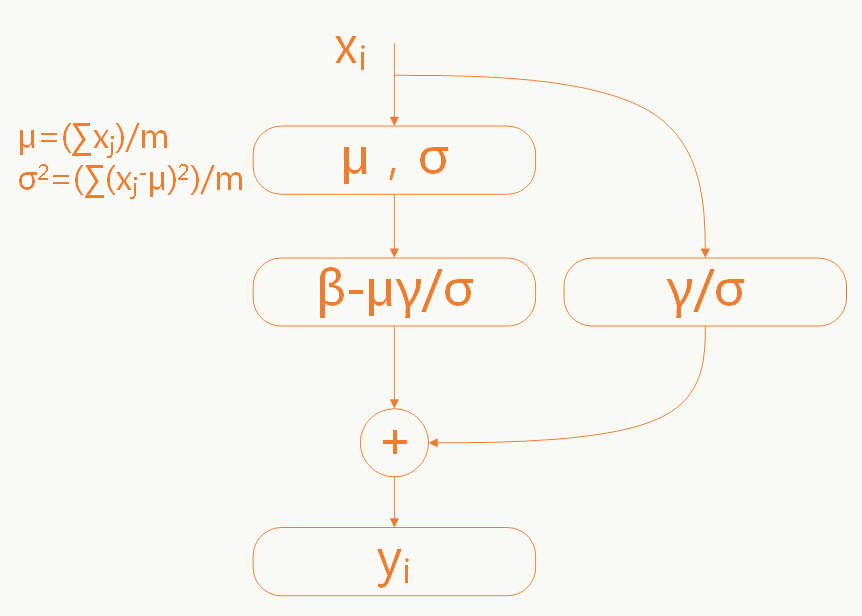
在模型Inference阶段,BN层需要的期望和方差是固定值,由于所有训练集batch的期望和方差已知,可以用这些值对整体训练集的期望和方差做无偏估计修正,修正方法为: \[ \begin{array}{l} E(x)=E_B(\mu_B)\\ Var(x)=\frac{m}{m-1}E_B(\sigma_B^2)\\ \text{其中B为训练集所有batch(大小都为m)的集合集合.}\\ \end{array} \]
Inference时的公式变为: \[ \begin{array}{l} y=\frac{\gamma}{\sqrt{Var(x)+\epsilon}}\cdot x+(\beta-\frac{\gamma E(x)}{\sqrt{Var(x)+\epsilon}}) \end{array} \]
5.13.3 卷积神经网络中的BN
卷积网络中采用权重共享策略,每个feature map只有一对\(\gamma\),\(\sigma\)需要学习。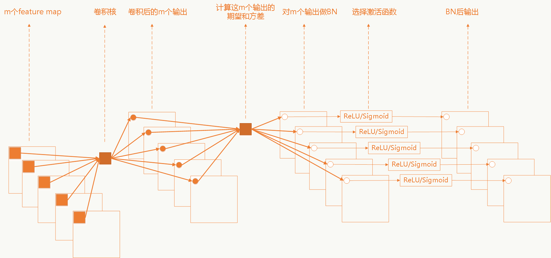
5.13.4 代码实践
1 | import copy |
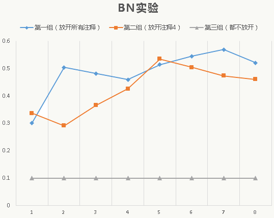
三组实验对比:
- 第一组:放开所有注释
- 第二组:放开注释4
- 第三组:注释掉所有BN
![]()
5.14 GoogLeNet Inception V3
GoogLeNet Inception V3在《Rethinking the Inception Architecture for Computer Vision》中提出(注意,在这篇论文中作者把该网络结构叫做v2版,我们以最终的v4版论文的划分为标准),该论文的亮点在于:
- 提出通用的网络结构设计准则
- 引入卷积分解提高效率
- 引入高效的feature map降维
5.14.1 网络结构设计的准则
前面也说过,深度学习网络的探索更多是个实验科学,在实验中人们总结出一些结构设计准则,但说实话我觉得不一定都有实操性:
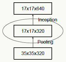
- 避免特征表示上的瓶颈,尤其在神经网络的前若干层 神经网络包含一个自动提取特征的过程,例如多层卷积,直观并符合常识的理解:如果在网络初期特征提取的太粗,细节已经丢了,后续即使结构再精细也没法做有效表示了;举个极端的例子:在宇宙中辨别一个星球,正常来说是通过由近及远,从房屋、树木到海洋、大陆板块再到整个星球之后进入整个宇宙,如果我们一开始就直接拉远到宇宙,你会发现所有星球都是球体,没法区分哪个是地球哪个是水星。所以feature map的大小应该是随着层数的加深逐步变小,但为了保证特征能得到有效表示和组合其通道数量会逐渐增加。 下图违反了这个原则,刚开就始直接从35×35×320被抽样降维到了17×17×320,特征细节被大量丢失,即使后面有Inception去做各种特征提取和组合也没用。
![]()
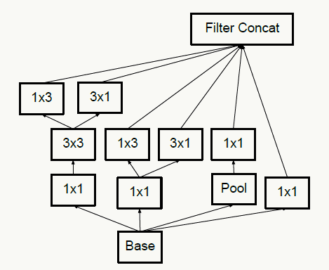
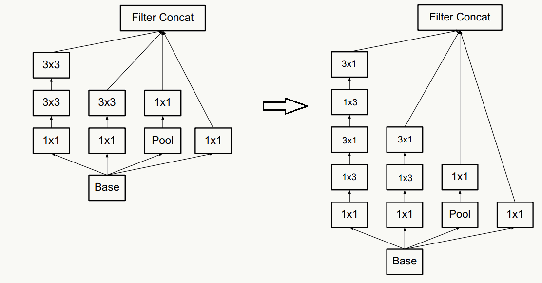
- 对于神经网络的某一层,通过更多的激活输出分支可以产生互相解耦的特征表示,从而产生高阶稀疏特征,从而加速收敛,注意下图的1×3和3×1激活输出:
![]()
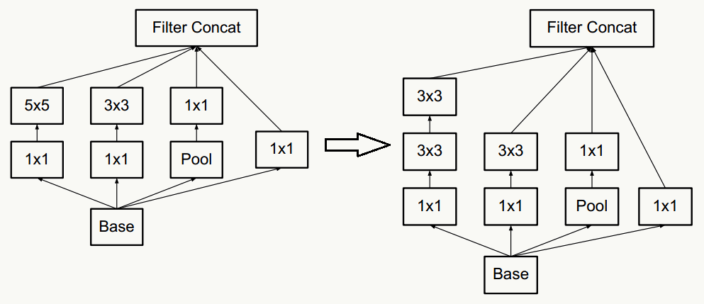
- 合理使用维度缩减不会破坏网络特征表示能力反而能加快收敛速度,典型的例如通过两个3×3代替一个5×5的降维策略,不考虑padding,用两个3×3代替一个5×5能节省1-(3×3+3×3)/(5×5)=28%的计算消耗。
![]()
- 通过合理平衡网络的宽度和深度优化网络计算消耗(这句话尤其不具有实操性)。
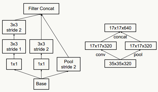
- 抽样降维,传统抽样方法为pooling+卷积操作,为了防止出现特征表示的瓶颈,往往需要更多的卷积核,例如输入为n个d×d的feature map,共有k个卷积核,pooling时stride=2,为不出现特征表示瓶颈,往往k的取值为2n,通过引入inception module结构,即降低计算复杂度,又不会出现特征表示瓶颈,实现上有如下两种方式:
![]()
5.14.2 平滑样本标注
对于多分类的样本标注一般是one-hot的,例如[0,0,0,1],使用类似交叉熵的损失函数会使得模型学习中对ground truth标签分配过于置信的概率,并且由于ground truth标签的logit值与其他标签差距过大导致,出现过拟合,导致降低泛化性。一种解决方法是加正则项,即对样本标签给个概率分布做调节,使得样本标注变成“soft”的,例如[0.1,0.2,0.1,0.6],这种方式在实验中降低了top-1和top-5的错误率0.2%。
5.14.3 网络结构
5.14.4 代码实践
为了能在单机跑起来,对feature map做了缩减,为适应cifar10的输入大小,对输入的stride做了调整,代码如下。
1 | # -*- coding: utf-8 -*- |
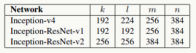
5.15 GoogLeNet Inception V4/ResNet V1/V2
这三种结构在《Inception-v4, Inception-ResNet and the Impact of Residual Connections on Learning》一文中提出,论文的亮点是:提出了效果更好的GoogLeNet Inception v4网络结构;与残差网络融合,提出效果不逊于v4但训练速度更快的结构。
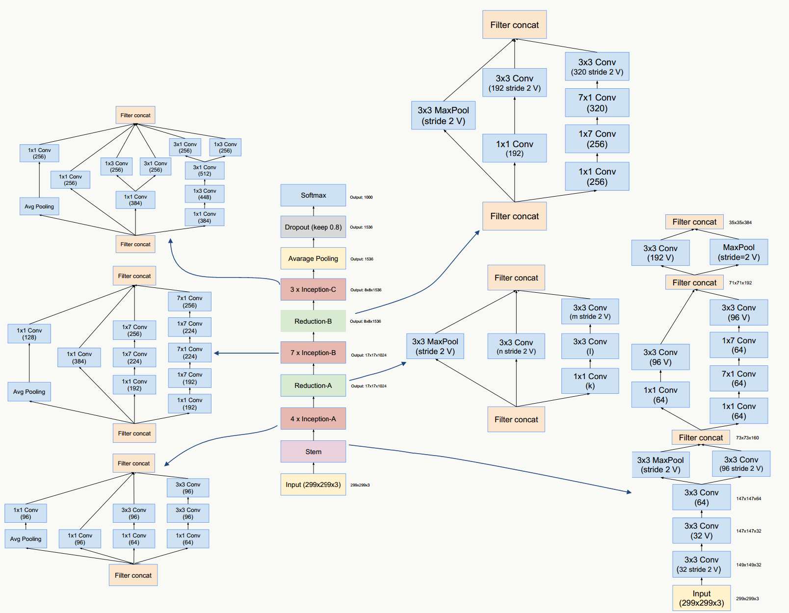
5.15.1 GoogLeNet Inception V4网络结构
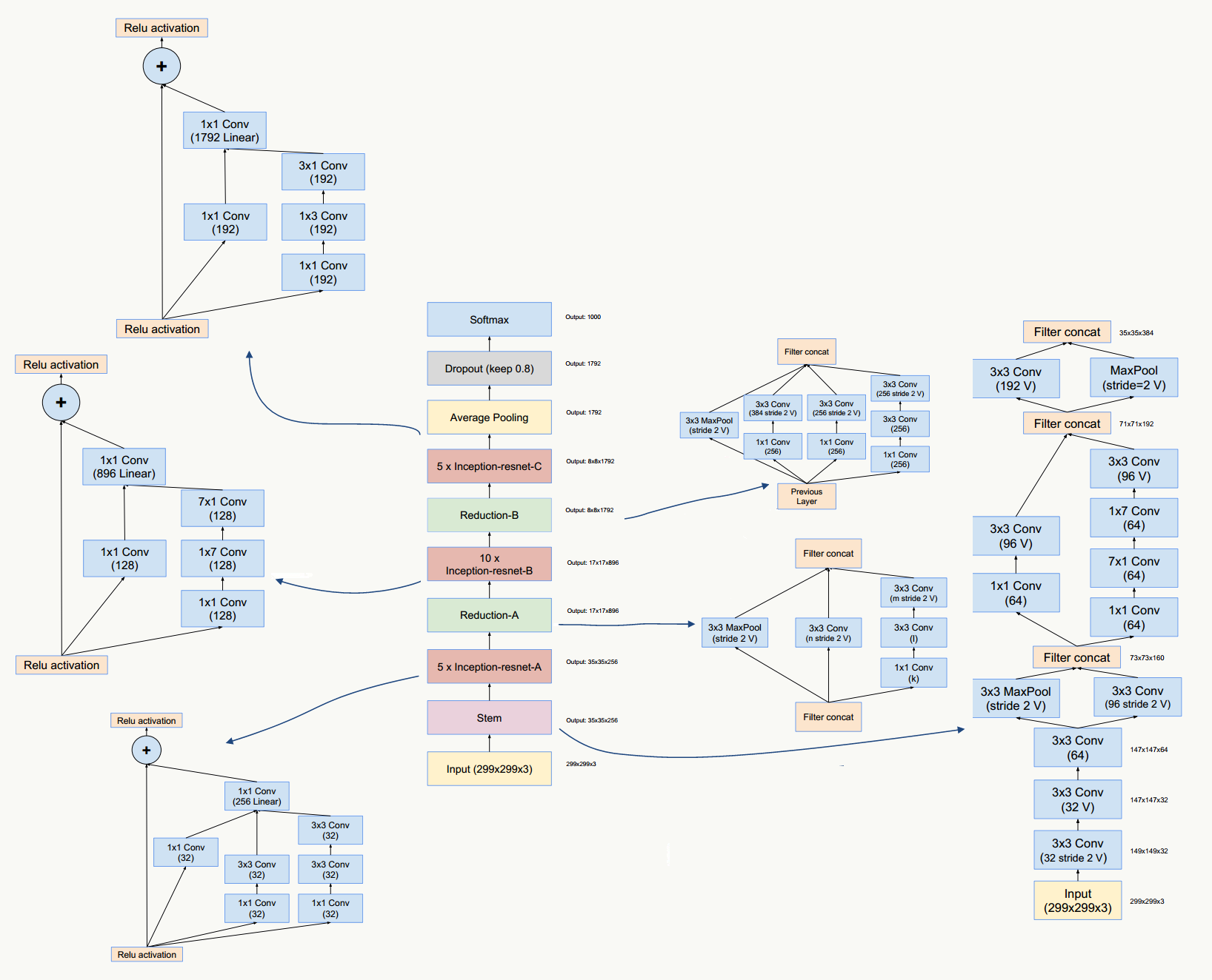
5.15.2 GoogLeNet Inception ResNet网络结构
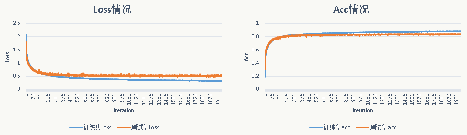
5.15.3 代码实践
GoogLeNet Inception ResNet V2
1 | # -*- coding: utf-8 -*- |
5.16 模型可视化
5.16.1 一些说明
神经网络本身包含了一系列特征提取器,理想的feature map应该是稀疏的以及包含典型的局部信息,通过模型可视化能有一些直观的认识并帮助我们调试模型,比如:feature map与原图很接近,说明它没有学到什么特征;或者它几乎是一个纯色的图,说明它太过稀疏,可能是我们feature map数太多了。可视化有很多种,比如:feature map可视化、权重可视化等等,我以feature map可视化为例。
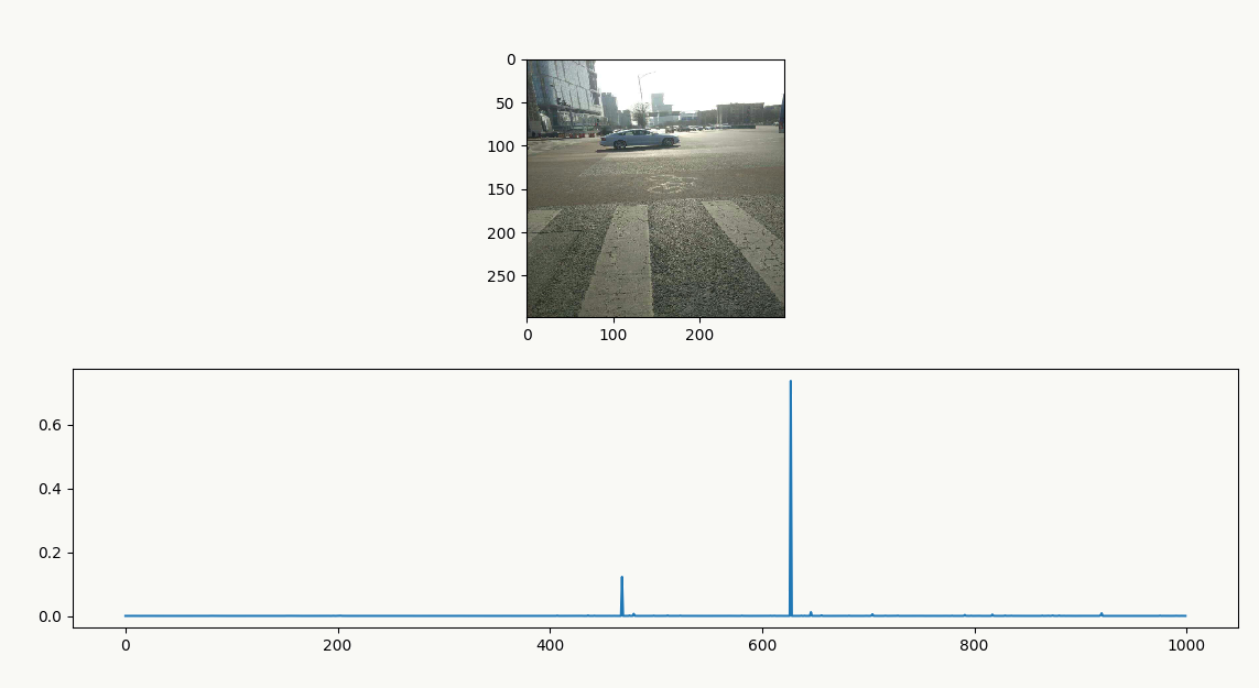
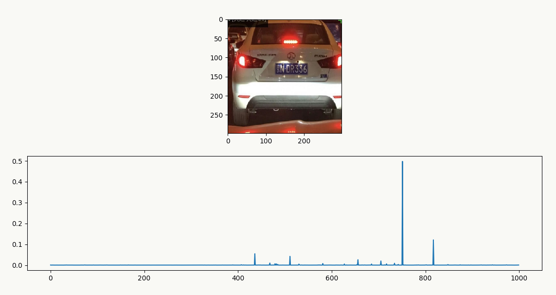
利用keras,采用在imagenet 1000分类的数据集上预训练好的googLeNet inception v3做实验,以下面两张图作为输入。
- 输入图片 奥迪A7及其分类结果:原图
![]()
![]()
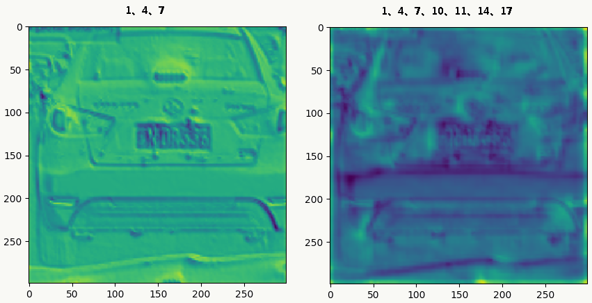
- feature map可视化 取网络的前15层,每层取前3个feature map。 奥迪A7 feature map:
![]()
![]()
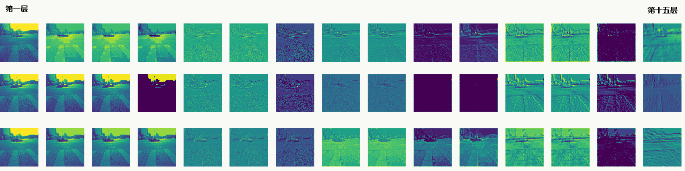
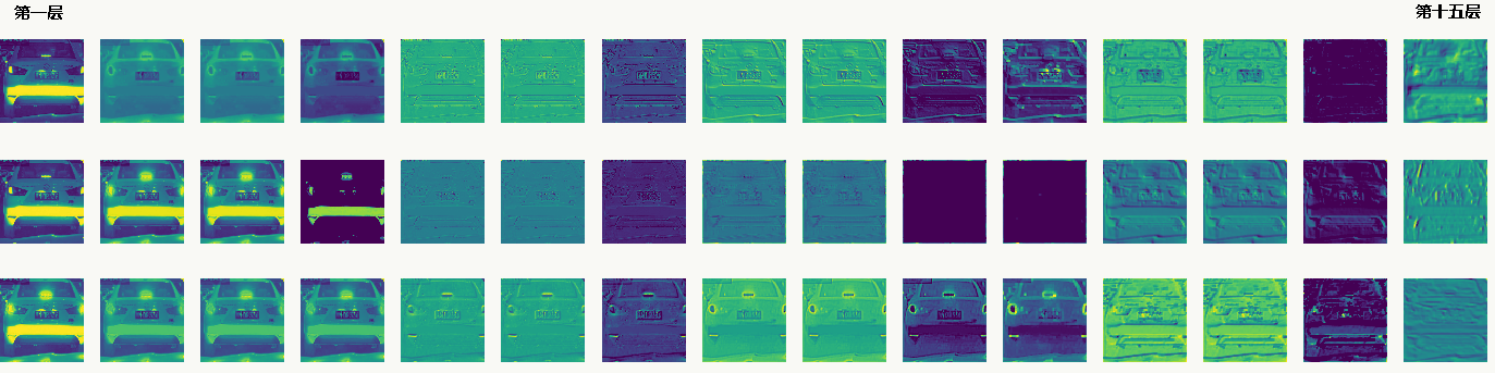
从左往右看,可以看到整个特征提取的过程,有的分离背景、有的提取轮廓,有的提取色差,但也能发现10、11层中间两个feature map是纯色的,可能这一层feature map数有点多了,另外北汽绅宝D50的光晕对feature map中光晕的影响也能比较明显看到。
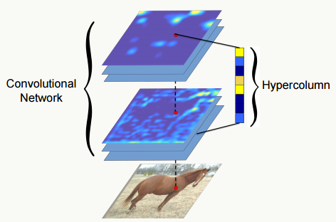
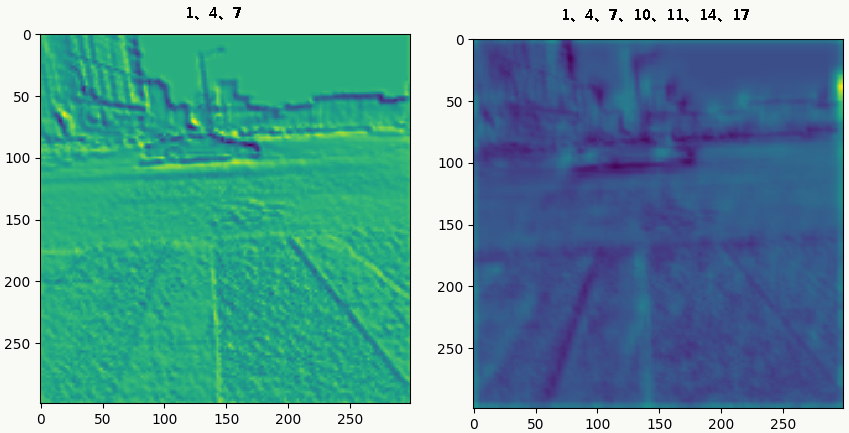
- Hypercolumns 通常我们把神经网络最后一个fc全连接层作为整个图片的特征表示,但是这一表示可能过于粗糙(从上面的feature map可视化也能看出来),没法精确描述局部空间上的特征,而网络的第一层空间特征又太过精确,缺乏语义信息(比如后面的色差、轮廓等),于是论文《Hypercolumns for Object Segmentation and Fine-grained Localization》提出一种新的特征表示方法:Hypercolumns——将一个像素的 hypercolumn 定义为所有 cnn 单元对应该像素位置的激活输出值组成的向量),比较好的tradeoff了前面两个问题,直观地看如图:
![]()
![]()
![]()
5.16.2 代码实践
需要安装opencv,注意它与python的版本兼容性,test_opencv函数可以测试是否安装成功。
1 | # -*- coding: utf-8 -*- |