9. 语义分割 9.1 FCN FCN在《Fully Convolutional Networks for Semantic Segmentation 》中第一次被提出,个人认为是实现图像end to end语义分割的开山之作,第一次做到了低成本的像素级分类预测(end-to-end, pixels-to-pixels),另外这个方法用在目标检测、识别上效果好于传统新方法(如:Faster R-CNN)。
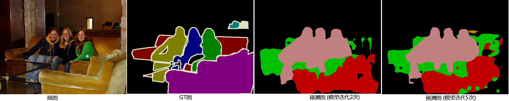
所谓语义分割简单说就是不但要知道你属于哪一类,还要知道你在哪儿:
从左到右分别是:原图、ground truth图、训练2轮的模型预测图、训练5轮的模型预测图(ps:截止本文前,训练达到理想状态还差200多轮)。
9.1.1 算法概述 CNN网络无疑是特征提取的利器,尤其在图像领域,回顾我们的做法:CNN做特征提取+全连接层做特征组合+分类/回归,为了能提高模型预测能力,需要通过多个全连接层(做笛卡尔积)做特征组合,这里是参数数量最多的地方,成为模型训练,尤其是inference时的最大瓶颈(所以模型压缩和剪枝算法会把第一把刀放在全连接层),而由于全连接层的存在,导致整个网络的输入必须是固定大小的:由于卷积和采样操作更本不关心输入大小如何,试想如果输入大小不一,不同图片到了全连接层时其输入节点数是不一样的,而网络的定义必须事先定义好,所以没法儿玩儿了,于是有了前面的SPP及RoI pooling来解决这个问题,FCN则是解决这个问题的另一个思路。
总结该算法要解决的问题如下:
1、取消网络对输入数据大小必须固定的限制;
2、提高模型效果且加快其训练和inference速度。
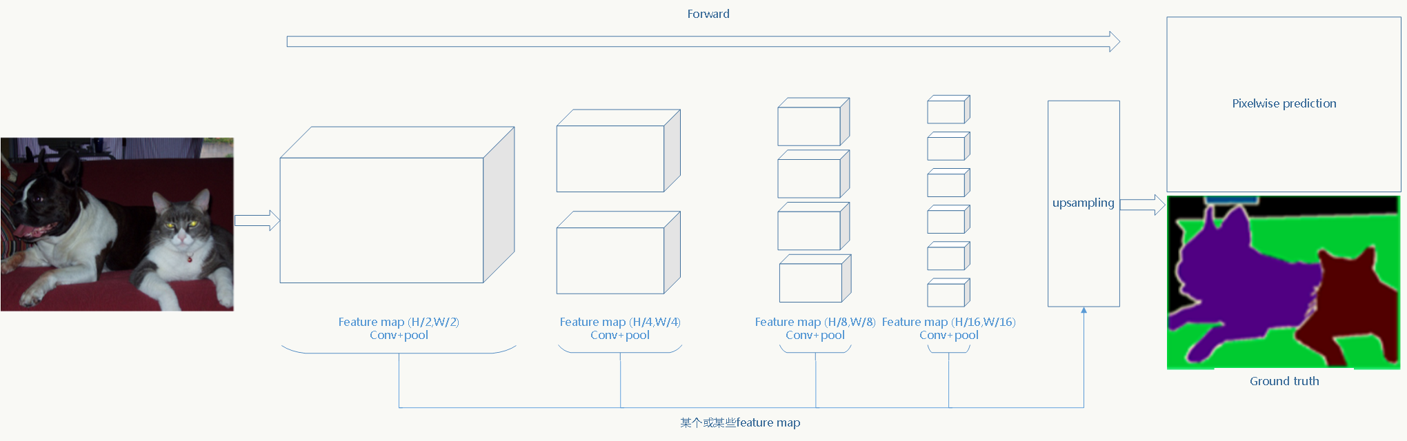
相比于传统CNN,FCN把全连接层全部替换成卷积层,并在feature map(可以是其中任何一个)上
做上采样 ,使其恢复到原始图片大小,这样不但保留了每个像素的空间信息,而且每个像素都会有一个分类预测。比如下图中pixelwise prediction那一层,小猫、小狗、电视、背景都会在像素级别做分类预测:
9.1.2 1×1卷积回顾 前面我们在介绍各种经典识别网络中介绍了1×1卷积核,回顾下它的作用,尤其对多通道而言:
1、每个1×1卷积核会有一个参数,利用它们可以做跨通道特征融合,即对多个通道的feature map做线性组合;
2、具有降维或升维作用,如:在GoogleNet中它可以跟在pooling层后面做降维,也可以直接通过减少通道数做降维,大大减少了参数量;
3、可以在不损失feature map信息的前提下利用后面的激活函数增加模型非线性表征能力,可以低成本的把网络变深。
9.1.3 全卷积网络 使用传统CNN做像素级分类的问题:
1、为了考虑上下文信息,需要一个滑动窗口,利用滑动窗口内的feature map对每个像素做分类,分类效果及存储空间随滑动窗口的大小上升;
2、为了考虑上下文信息,导致相邻两个窗口之间有大量的像素重复,意味着大量计算重复;
3、原图的空间信息没有被很好的利用;
4、原图需要固定大小,图像的resize(本质就是图像的下采样)导致信息损失。
FCN则很好的解决了上面几个问题。
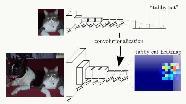
上图是传统CNN工作流程,下图是FCN工作流程,它最终可以得到关于目标的热图,这种变换除了在语义分割、检测、识别上用到,也会在feature map可视化上用来帮助分析特征。 一张图说明:
理解FCN最关键的一步是理解上采样(upsampling)。
9.1.4 Nyquist–Shannon采样定理 关于采样,这个话题可大可小,从定义上说,采样是这么一个过程:在尽可能减少信息损失的情况下,将信号从一种采样率下的形态转换为另外一种,对于图片,这个过程叫做图像缩放。详细定义参见Resampling 。
对计算机而言无法处理连续信号(读者想想为什么?),必须通过采样做信号离散化,那就必须回答一个问题:理想情况下,以什么样的频率采样能完美重构连续信号的信息。
Nyquist–Shannon采样定理回答了上面的问题:当对信号均匀间隔离散采样且信号的带宽小于采样率的一半时,原始连续信号可以被其得到的采样样本完全重构,不满足该条件则会出现混叠(Aliasing)现象。
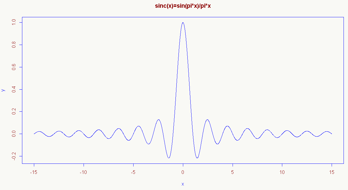
理论上连续信号可以通过以下公式重构(信息重构器):
\[ \text{s(x) = sum_n s(n*T) * sinc((x-n*T)/T), with sinc(x) = sin(pi*x)/(pi*x) for x!=0, and = 1 for x=0} \] 其中采样率为:1/T,s(n*T)是s(x)的采样样本,sinc(x)是采样核(resampling kernel)。
一般来说 信息重构器有以下性质:
1、\(s(m*T)\) 确实是信号\(s(x)\) 的样本;
2、$_n{sinc((x-n*T)/T)} = 1 $;
3、resampling kernel:\(sinc(x)=* \text{ for x!=0, and = 1 for x=0}\) ;
4、resampling kernel:\(sinc(x)\) 是对称的,\(sinc(x) = sinc(-x)\) ;
5、resampling kernel:\(sinc(x)\) 是处处可微的。
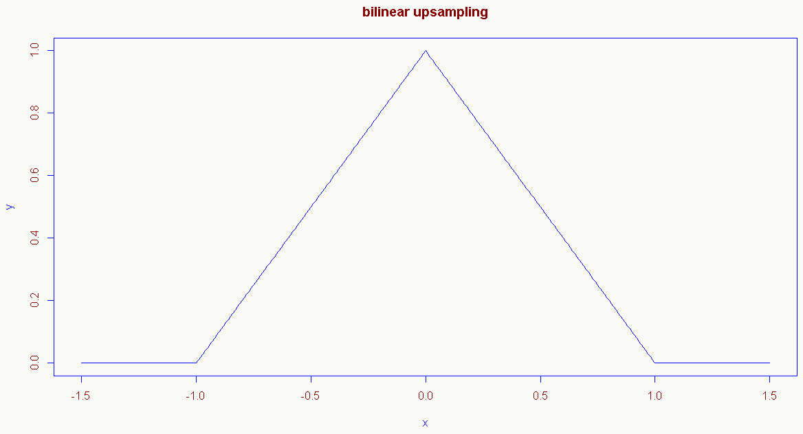
当然还有其他形式的resampling kernel,比如bilinear resampling kernel,满足上述性质2、3、4:
\[ f(x)= \begin{cases} 1 - |x|& \text{|x|<1}\\ 0& \text{other} \end{cases} \]
这个函数在FCN里广泛用到。
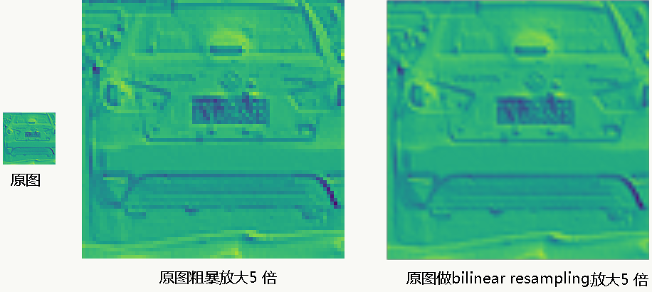
我利用scikit-image library给个简单的bilinear resampling示例:
1
2
3
4
5
6
7
8
9
10
11
12
13
14
15
16
17
18
19
20
21
22
23
import skimage.transformfrom numpy import ogrid, repeat, newaxisfrom skimage import iodef upsample_with_skimage (img, factor ): return skimage.transform.rescale(img, factor, mode='constant' , cval=0 , order=1 ) if __name__ == '__main__' : target = upsample_with_skimage(img=io.imread("feature_map.jpg" ), factor=5 ) io.imsave("upsampling.png" , target, interpolation='none' )
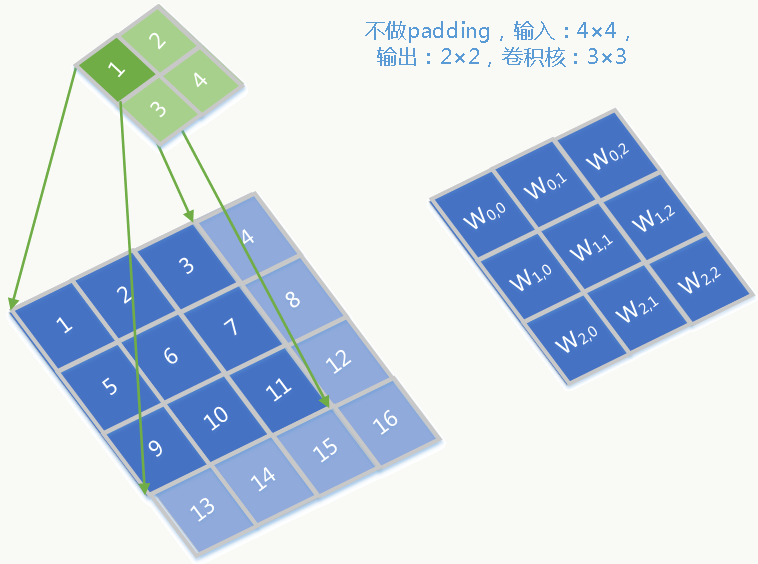
9.1.5 转置卷积(Transposed Convolution) 很多人把这个过程叫做“反卷积(deconvolution)”,但我认为这么叫是错误的,它的过程并不是对卷积的逆运算,它除了用在FCN中还会用在卷积可视化、对抗神经网络中。 原理如下:
假设,输入为4×4、输出为2×2、卷积核为3×3,则把输出、输入和卷积核按照从左到右、从上到下展开为向量,前向传播的卷积过程相当于输入与以下稀疏矩阵的乘积:
\[ \begin{equation} W=\left( \begin{array}{lll} w_{0,0} &0&0&0 \\ w_{0,1} &w_{0,0}&0&0 \\ w_{0,2} &w_{0,1}&0&0 \\ 0 &w_{0,2}&0&0 \\ w_{1,0} &0&w_{0,0}&0 \\ w_{1,1} &w_{1,0}&w_{0,1}&w_{0,0} \\ w_{1,2} &w_{1,1}&w_{0,2}&w_{0,1} \\ 0 &w_{1,2}&0&w_{0,2} \\ w_{2,0} &0&w_{1,0}&0 \\ w_{2,1} &w_{2,0}&w_{1,1}&w_{1,0} \\ w_{2,2} &w_{2,1}&w_{1,2}&w_{1,1} \\ 0 &w_{2,2}&0&w_{1,2} \\ 0 &0&w_{2,0}&0 \\ 0 &0&w_{2,1}&w_{2,0} \\ 0 &0&w_{2,2}&w_{2,1} \\ 0 &0&0&w_{2,2} \end{array} \right)^T\nonumber \end{equation} \]
前向传播过程就表述为:
\[ \begin{equation} Y=W \cdot X =\left( \begin{array}{lll} w_{0,0} &0&0&0 \\ w_{0,1} &w_{0,0}&0&0 \\ w_{0,2} &w_{0,1}&0&0 \\ 0 &w_{0,2}&0&0 \\ w_{1,0} &0&w_{0,0}&0 \\ w_{1,1} &w_{1,0}&w_{0,1}&w_{0,0} \\ w_{1,2} &w_{1,1}&w_{0,2}&w_{0,1} \\ 0 &w_{1,2}&0&w_{0,2} \\ w_{2,0} &0&w_{1,0}&0 \\ w_{2,1} &w_{2,0}&w_{1,1}&w_{1,0} \\ w_{2,2} &w_{2,1}&w_{1,2}&w_{1,1} \\ 0 &w_{2,2}&0&w_{1,2} \\ 0 &0&w_{2,0}&0 \\ 0 &0&w_{2,1}&w_{2,0} \\ 0 &0&w_{2,2}&w_{2,1} \\ 0 &0&0&w_{2,2} \end{array} \right)^T\nonumber \cdot \left( \begin{array}{lll} 1\\ 2\\ 3\\ 4 \\ 5\\ 6\\ 7\\ 8 \\ 9\\ 10\\ 11\\ 12\\ 13\\ 14\\ 15\\ 16 \end{array} \right)\nonumber= \left( \begin{array}{lll} 1\\ 2\\ 3\\ 4 \end{array} \right)\nonumber \end{equation} \]
误差反向传播(如果记不清了可以回看5.1节):
\[ \frac{\partial E}{\partial X}=W^T\frac{\partial E}{\partial Y} \]
那么反过来,我们希望从4维向量映射回16维向量怎么做呢:把上面过程逆反一下(当然该做padding还得做): 前向传播: \[Y=W^T X \] 反向传播: \[ \frac{\partial E}{\partial X}=(W^T)^T\frac{\partial E}{\partial Y}=W\frac{\partial E}{\partial Y} \]
整个过程平滑柔顺,多种情况下的详细解释可以看:《Convolution arithmetic tutorial》
keras下做转置卷积,输入feature map及最终效果同8.7.4。
1 2 3 4 5 6 7 8 9 10 11 12 13 14 15 16 17 18 19 20 21 22 23 24 25 26 27 28 29 30 31 32 33 34 35 36 37 38 39 40 41 42 43 44 45 46 47 48 49 50 51 52 53 54 55 56 57 58 59 60 61 62 63 64 65 66 67 68 69 70 71 72 73 74 75 76 77 78 79 80 81 82 83 from __future__ import divisionimport numpy as npimport tensorflow as tffrom skimage import ioimport skimageimport ioimport osimport keras.backend as Kdef get_kernel_size (factor ): """ 给定上采样因子,返回核大小,上采样因子大小等于转置卷积步长。 """ return 2 * factor - factor % 2 def upsample_filt (size ): """ 返回上采样bilinear kernel矩阵。 """ factor = (size + 1 ) // 2 if size % 2 == 1 : center = factor - 1 else : center = factor - 0.5 og = np.ogrid[:size, :size] return (1 - abs (og[0 ] - center) / factor) * \ (1 - abs (og[1 ] - center) / factor) def bilinear_upsample_weights (factor, channel ): """ 使用bilinear filter初始化转置卷积权重矩阵。 """ filter_size = get_kernel_size(factor) weights = np.zeros((filter_size, filter_size, channel, channel), dtype=np.float32) upsample_kernel = upsample_filt(filter_size) for i in xrange(channel): weights[:, :, i, i] = upsample_kernel return weights def upsample_keras (factor, input_img ): SCALE = 256 channel = input_img.shape[2 ] scale_height = input_img.shape[0 ] * factor scale_width = input_img.shape[1 ] * factor expanded_img = np.expand_dims(input_img, axis=0 ) with tf.device("/gpu:1" ): gpu_options = tf.GPUOptions(per_process_gpu_memory_fraction=1 , allow_growth=True ) os.environ["CUDA_VISIBLE_DEVICES" ] = "1" sess = tf.Session(config=K.tf.ConfigProto(allow_soft_placement=True , log_device_placement=True , gpu_options=gpu_options)) input_value = tf.placeholder(tf.float32) trans_filter = tf.placeholder(tf.float32) upsample_filter_np = bilinear_upsample_weights(factor, channel) res = K.conv2d_transpose(input_value, trans_filter, output_shape=[1 , scale_height, scale_width, channel], padding='same' , strides=(factor, factor)) final_result = sess.run(res, feed_dict={trans_filter: upsample_filter_np, input_value: expanded_img}) if channel != 1 : return final_result.squeeze() / SCALE return final_result.squeeze() upsampled_img_keras = upsample_keras(factor=5 , input_img=skimage.io.imread("feature_map.jpg" )) skimage.io.imsave("bilinear_feature_map.jpg" ,upsampled_img_keras, interpolation='none' )
9.1.6 代码实践 开源代码可参见:Keras-FCN ,虽然缺点是训练有点慢,模型有点大,但对于理解如何实现很有帮助。
里面实现了五种模型,两种基于vgg-16,两种基于resnet-50,一种基于densenet。
上采样操作做为一个新的网络层意味着它需要能够前向传播、反向传播、更新权重,其实现在代码中为BilinearUpSampling.py。
inference.py的代码需要稍微变下:
1
2
3
4
5
6
7
8
9
10
11
12
13
14
15
16
17
18
19
20
21
22
23
24
25
26
27
28
29
30
31
32
33
34
35
36
37
38
39
40
41
42
43
44
45
46
47
48
49
50
51
52
53
54
55
56
57
58
59
60
61
62
63
64
65
66
67
68
69
70
71
72
73
74
75
76
77
78
79
80
81
82
83
84
85
86
87
88
89
90
91
92
93
94
95
import numpy as npimport matplotlib.pyplot as pltfrom pylab import *import osimport sysimport cv2from PIL import Imagefrom keras.preprocessing.image import *from keras.models import load_modelimport keras.backend as Kfrom keras.applications.imagenet_utils import preprocess_inputfrom models import *def inference (model_name, weight_file, image_size, image_list, data_dir, label_dir, return_results=True , save_dir=None , label_suffix='.png' , data_suffix='.jpg' ): current_dir = os.path.dirname(os.path.realpath(__file__)) batch_shape = (1 , ) + image_size + (3 , ) save_path = os.path.join(current_dir, 'Models/' +model_name) model_path = os.path.join(save_path, "model.json" ) checkpoint_path = os.path.join(save_path, weight_file) model = globals ()[model_name](batch_shape=batch_shape, input_shape=(512 , 512 , 3 )) model.load_weights(checkpoint_path, by_name=True ) model.summary() results = [] total = 0 for img_num in image_list: img_num = img_num.strip('\n' ) total += 1 print ('#%d: %s' % (total,img_num)) image = Image.open ('%s/%s%s' % (data_dir, img_num, data_suffix)) image = img_to_array(image) label = Image.open ('%s/%s%s' % (label_dir, img_num, label_suffix)) label_size = label.size img_h, img_w = image.shape[0 :2 ] pad_w = max (image_size[1 ] - img_w, 0 ) pad_h = max (image_size[0 ] - img_h, 0 ) image = np.lib.pad(image, ((pad_h/2 , pad_h - pad_h/2 ), (pad_w/2 , pad_w - pad_w/2 ), (0 , 0 )), 'constant' , constant_values=0. ) '''img = array_to_img(image, 'channels_last', scale=False) img.show() exit()''' image = np.expand_dims(image, axis=0 ) image = preprocess_input(image) result = model.predict(image, batch_size=1 ) result = np.argmax(np.squeeze(result), axis=-1 ).astype(np.uint8) result_img = Image.fromarray(result, mode='P' ) result_img.palette = label.palette result_img = result_img.crop((pad_w/2 , pad_h/2 , pad_w/2 +img_w, pad_h/2 +img_h)) if return_results: results.append(result_img) if save_dir: result_img.save(os.path.join(save_dir, img_num + '.png' )) return results if __name__ == '__main__' : with tf.device('/gpu:1' ): gpu_options = tf.GPUOptions(per_process_gpu_memory_fraction=1 , allow_growth=True ) os.environ["CUDA_VISIBLE_DEVICES" ] = "1" tf.Session(config=K.tf.ConfigProto(allow_soft_placement=True , log_device_placement=True , gpu_options=gpu_options)) model_name = 'AtrousFCN_Resnet50_16s' weight_file = 'checkpoint_weights.hdf5' image_size = (512 , 512 ) data_dir = os.path.expanduser('~/.keras/datasets/VOC2012/VOCdevkit/VOC2012/JPEGImages' ) label_dir = os.path.expanduser('~/.keras/datasets/VOC2012/VOCdevkit/VOC2012/SegmentationClass' ) image_list = sys.argv[1 :] results = inference(model_name, weight_file, image_size, image_list, data_dir, label_dir, save_dir="result" ) for result in results: result.show(title='result' , command=None )
9.2 FCN-CRF 9.3 SegNet 9.4 UberNet 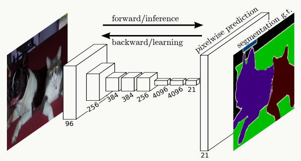 本章对于机器学习在计算机视觉中的语义分割领域经典的FCN模型做了简要介绍,后几节待填坑。